Manual for solving typed problems in Microsoft Excel
Good afternoon, dear habrozhiteli!
From time to time, some (and maybe more than some) of us have to deal with the tasks of processing small amounts of data, ranging from the preparation and analysis of the household budget to any calculations for work, study, etc. Perhaps the most suitable tool for this is Microsoft Excel (or perhaps its other counterparts, but they are less common).
The search gave me just one article on Habré on a similar topic - “Talmud using Google SpreadSheet formulas” . It gives a good description of the basic things to work in excel (although it’s not 100% about excel itself).
')
Thus, having accumulated a certain pool of requests / tasks, an idea appeared to type them and propose possible solutions (though not all possible, but quickly giving a result).
It will be about solving the most common tasks faced by users.
The description of the solutions is constructed as follows - a case containing the original task is given, which is gradually becoming more complex, a detailed solution with explanations is given for each step. The names of the functions will be given in Russian, but in parentheses, when first mentioned, the original name in English will be given (as the experience of the overwhelming majority of users has the Russian version installed).
Case_1: Logic and match functions
“I have a set of values in the table and it is necessary that when a certain condition / set of conditions is fulfilled, a certain value is displayed”
Data is usually presented in tabular form:
Condition:
The “IF” (IF) formula will help us in this, which refers to logical formulas and can produce in the solution any values that we write in advance in the formula. Please note that any text values are written using quotes.
The formula syntax is as follows:
IF (log_expression, [value_if_fresh_tour], [value_if_fold_])
The syntax for the formula to solve is:
Displaying the result in cell D2:
At the output we get the result:

It happens that the condition is more complex, for example the implementation of 2 or more conditions:
In this case, we can no longer restrict ourselves to the use of the formula “IF” alone; we need to add another formula to its syntax. And it will be another logical formula "AND" (AND).
The formula syntax is as follows:
And (logical_value1, [logical_value2], ...)
The solution syntax is as follows:
Displaying the result in cell D2:
Thus, using a combination of 2 formulas, we find the solution to our problem and get the result:
Let's try to complicate the task - a new condition:
The solution syntax is as follows:
Displaying the result in cell D2:
As can be seen from the record, one condition “OR” (OR) and two conditions are included in the “IF” formula using the “AND” formula included in it. If at least one of the conditions of the 2nd level is “TRUE”, then the result will be “1” in the column “Result”, otherwise it will be “0”.
Result:
We now turn to the following situation:
Imagine that, depending on the value in the column “Condition”, a certain condition should be displayed in the column “Result”, below is the correspondence between the values and the result.
Condition:
When solving a problem using the IF function, the syntax is as follows:
Outputting the result to cell B2:
Result:
As you can see, writing such a formula is not only not very convenient and cumbersome, but it may take some time for an inexperienced user to edit it in case of an error.
The disadvantage of this approach is that it is applicable for a small number of conditions, because all of them will have to be typed manually and “inflate” our formula to large sizes, however the approach is distinguished by complete “omnivorousness” to values and universality of use.
Alternative solution_1:
Using the formula "CHOICE" (CHOOSE),
Function syntax:
SELECT (index_number, value1, [value2], ...)
When using it, we immediately record the results of the conditions depending on the specified values.
Condition:
Formula syntax:
The result is similar to the solution with the chain of IF functions above.
When applying this formula, there are the following limitations:
Only digits can be indicated in the “A2” cell (index number), and the result values will be displayed in ascending order from 1 to 254 values.
In other words, the function will work only if the cell “A2” indicates the numbers from 1 to 254 in ascending order and this imposes certain restrictions when using this formula.
Those. if we want, what would the value of "G" be displayed when specifying the number 5,
then the formula will have the following syntax:
Outputting the result to cell B2:
As you can see, the value “4” in the formula we have to leave empty and transfer the result “G” to the sequence number “5”.
Alternative solution_2:
Here we come to one of the most popular functions of Excel, the mastering of which automatically turns any office worker into an “advanced user excel” / sarcasm /.
Formula syntax:
CRF (lookup_value, table, column_number, [interval_view])
Important: the “CDF” function searches for a match only by the first unique record, if the desired_value is present in the “Table” argument several times and has different values, the “CDF” function will find only the FIRST match, the results for all other matches will not be shown. VLOOKUP ”(VLOOKUP) is associated with another approach to working with data, namely the formation of“ directories ”.
The essence of the approach is to create a “directory” of matching the “Searched_value” argument to a specific result, separately from the main array, in which the conditions and the corresponding values are written:
Then, in the working part of the table, the formula is already written with reference to the reference book that was filled out earlier. Those. in the directory in the “D” column, a value is searched from the “A” column, and when a match is found, the value from the “E” column is displayed in the “B” column.
Formula syntax:
Outputting the result to cell B2:
Result :
Now imagine a situation where you need to pull the data into one table from another, while the tables are not identical. See example below.
It can be seen that the rows in the columns “Product” of both tables do not match, however, this is not an obstacle to the use of the “CDF” function.
Outputting the result to cell B2:
But when solving, we encounter a new problem - when “pulling” the formula we wrote to the right from column “B” to column “E”, we will have to manually replace the argument “column_number”. This is a laborious and ungrateful business, because another function, COLUMN, comes to the rescue.
Function syntax:
COLUMN ([link])
If you use an entry like:
then the function will display the number of the current column (in the cell of which the formula is written).
The result is a number that can be used in the “CDF” function, which we will use and get the following formula entry:
Outputting the result to cell B2:
The COLUMN function determines the number of the current column that will be used by the column_number argument to determine the number of the search column in the directory.
In addition, you can use the design:
Instead of the number “1”, you can use any number (and not only subtract it, but also add it to the value obtained) to get the desired result if you don’t want to refer to a specific cell in the column with the number we need.
The result is:
We continue to develop the topic and complicate the condition: imagine that we have two directories with different data on products and it is necessary to display in the table with the result values depending on what type of directory is specified in the column "Reference"
Condition:
The solution that immediately comes to mind is:
Displaying the result in cell C3:
Pros : the name of the directory can be any (text, numbers, and their combination), cons - not very good if there are more than 3 options.
If directory numbers are always numbers, it makes sense to use the following solution:
Displaying the result in cell C3:
Pros : the formula can include up to 254 reference books, minuses - their name must be strictly numeric.
Result for the formula using the “SELECT” function:
Bonus: CDF on two or more signs in the argument "is_value".
Condition:
Both tables are shown below:
As can be seen from the tabular forms, each position has not only the name (which is not unique), but also belongs to a certain class and has its own packaging option.
Using a combination of name and class and packing, we can create a new sign, for this in the table with data we create an additional column “Additional attribute”, which we fill in using the following formula:
Using the “&” symbol, we combine three signs into one (the separator between words can be any, as well as not be at all, the main thing is to use a similar rule for searching)
The analogue of the formula can be the function "CONCATENATE", in this case it will look like this:
After the additional attribute is created for each record in the table with data, we start writing the search function for this attribute, which will look like:
Displaying the result in cell D3:
In the function “CDF”, we use the same combination of three attributes (name_class_packing) as the “search_value” argument, but take it in the table to fill it and enter it directly into the argument (alternatively, we could select the value for the argument in an additional column in table for filling, but this action will be redundant).
I remind you that the use of the IFERROR function (IFERROR) is necessary if the desired value is not found, and the CDF function will display the meaning of "# N / A" (see below).
The result in the picture below:
This technique can be used for more signs, the only condition is the uniqueness of the resulting combinations, if it is not respected, the result will be incorrect.
Case_3 Search for a value in an array, or when CDF is unable to help us
Consider the situation when it is necessary to understand whether there are necessary values in the array of cells.
Task:
Visually, everything looks like this:
As we can see, the “CDF” function is powerless here, since we are not looking for an exact match, but the presence of the desired value in the cell.
To solve the problem, it is necessary to use a combination of several functions, namely:
"IF A"
"ERROR"
"LINE"
"TO FIND"
In order of all, "IF" we have already disassembled earlier, because we move on to the function "ERROR" (IFERROR)
Important: this formula is almost always required when working with arrays of information and reference books, because it is often the case that the sought value is not in the directory and in this case the function returns an error. If an error is displayed in the cell and the cell participates, for example, in the calculation, then it will also happen with an error. Plus, cells where the formula returned an error can be assigned different values, which facilitate their statistical processing. Also, in the event of an error, you can perform other functions, which is very convenient when working with arrays and allows you to build formulas taking into account fairly extensive conditions.
"LOWER" (LOWER)
Important: the function "LINE" does not replace characters that are not letters.
The role in the formula: since the FIND function (FIND) searches for and takes into account the case of the text, it is necessary to bring all the text to one register, otherwise the tea will not equal tea, etc. This is relevant if the register value is not a condition for searching and selecting values; otherwise, the “LINE” formula can be omitted, so the search will be more accurate.
Now more about the syntax of the function "FIND" (FIND).
The syntax of the formula-solution will be:
Outputting the result to cell B2:
Let us analyze the logic of the formula for the actions:
As can be seen from the figure above, thanks to the "LINE" and "FIND" functions, we find the desired values regardless of the case of the characters and the location in the cell, but it is necessary to pay attention to line 5.
The search condition is set as “111”, but the search array has the value “1111111 cookies”, but the formula gives the result “Bingo!”. This is because the value "111" is included in the series of values "1111111", as a result there is a match. In the opposite case, this condition will not work.
Case_4 Search for a value in an array on several conditions, or when CDF is all the more unable to help us
, « » «» , «» «».
:
:
«» «»
«» (INDEX)
«» , , «_» «_».
«» (MATCH)
The FIND function searches for the specified element in a range of cells and returns the relative position of that element in the range.
The essence of the use of the combination of the functions "INDEX" and "MATCH" in fact, we search for the coordinates of values by their name on the "coordinate axes".
The Y axis will be the “Name” column, and the X axis will be the “Months” row.
part of the formula:
:
, (1; #/) «» «».
B4 :
, , :
, «_» «#/», «B4» .
, «#/», .
Result:
«», , , «0», :
B4:
:
, «#/» .
_5
, , .
:

(LOOKUP) , . : .
B3:

«_» «_» – Excel.
:
B3:
=(E3;{0;1001;1501;2001;2501};{«»;«»;«»;«»;«»})
_6
:
(SUMIF) –
(SUMIFS) –
(SUMPRODUCT) –
«» (SUM) , «» :
({=(()*())}
«»
«»:
:

, , , .
, «» .
B4:
:
, , .
Result:
, «» «» «», «» , « »:
B4:
:
:
:
, / , , , , .
Result:

, , , - , ( ).
, - Excel, , !
!
From time to time, some (and maybe more than some) of us have to deal with the tasks of processing small amounts of data, ranging from the preparation and analysis of the household budget to any calculations for work, study, etc. Perhaps the most suitable tool for this is Microsoft Excel (or perhaps its other counterparts, but they are less common).
The search gave me just one article on Habré on a similar topic - “Talmud using Google SpreadSheet formulas” . It gives a good description of the basic things to work in excel (although it’s not 100% about excel itself).
')
Thus, having accumulated a certain pool of requests / tasks, an idea appeared to type them and propose possible solutions (though not all possible, but quickly giving a result).
It will be about solving the most common tasks faced by users.
The description of the solutions is constructed as follows - a case containing the original task is given, which is gradually becoming more complex, a detailed solution with explanations is given for each step. The names of the functions will be given in Russian, but in parentheses, when first mentioned, the original name in English will be given (as the experience of the overwhelming majority of users has the Russian version installed).
Case_1: Logic and match functions
“I have a set of values in the table and it is necessary that when a certain condition / set of conditions is fulfilled, a certain value is displayed”
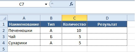
Data is usually presented in tabular form:
Condition:
- if the value in the "Quantity" column is greater than 5,
- then you need to display in the "Result" column the value "Order not required",
The “IF” (IF) formula will help us in this, which refers to logical formulas and can produce in the solution any values that we write in advance in the formula. Please note that any text values are written using quotes.
The formula syntax is as follows:
IF (log_expression, [value_if_fresh_tour], [value_if_fold_])
- Log_expression is an expression that results in the value TRUE or FALSE.
- Value_if_status is the value that is displayed if the logical expression is true
- Value_if_fold is the value that is output if the logical expression is false
The syntax for the formula to solve is:
Displaying the result in cell D2:
= IF (C5> 5; “Order Not Required”; “Order Required”)
At the output we get the result:
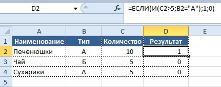
It happens that the condition is more complex, for example the implementation of 2 or more conditions:
- if the value in the “Quantity” column is greater than 5, and the value in the “Type” column is “A”
- then it is necessary to output the value “1” in the column “Result”, otherwise “0”.
In this case, we can no longer restrict ourselves to the use of the formula “IF” alone; we need to add another formula to its syntax. And it will be another logical formula "AND" (AND).
The formula syntax is as follows:
And (logical_value1, [logical_value2], ...)
- Logical_value1-2 etc. - verifiable condition, the calculation of which gives the value TRUE or FALSE
The solution syntax is as follows:
Displaying the result in cell D2:
= IF (AND (C2> 5; B2 = “A”); 1; 0)
Thus, using a combination of 2 formulas, we find the solution to our problem and get the result:
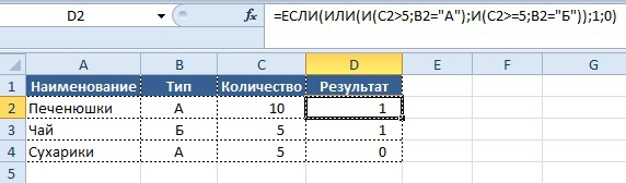
Let's try to complicate the task - a new condition:
- if the value in the “Quantity” column is 10, and the value in the “Type” column is “A”
- or the value in the "Quantity" column is greater than or equal to 5, and the value of "Type" is equal to "B"
- then it is necessary to output the value “1” in the column “Result”, otherwise “0”.
The solution syntax is as follows:
Displaying the result in cell D2:
= IF (OR (AND (C2 = 10; B2 = "A"); AND (C2> = 5; B2 = "B"); 1; 0)
As can be seen from the record, one condition “OR” (OR) and two conditions are included in the “IF” formula using the “AND” formula included in it. If at least one of the conditions of the 2nd level is “TRUE”, then the result will be “1” in the column “Result”, otherwise it will be “0”.
Result:
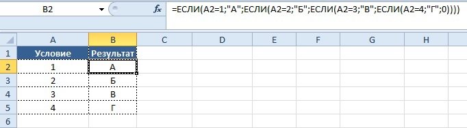
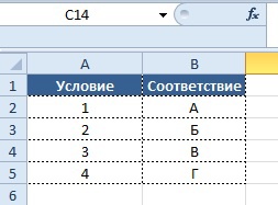
We now turn to the following situation:
Imagine that, depending on the value in the column “Condition”, a certain condition should be displayed in the column “Result”, below is the correspondence between the values and the result.
Condition:
- 1 = A
- 2 = B
- 3 = B
- 4 = G
When solving a problem using the IF function, the syntax is as follows:
Outputting the result to cell B2:
= IF (A2 = 1; "A"; IF (A2 = 2; "B"; IF (A2 = 3; "C"; IF (A2 = 4; "D"; 0)))
Result:
As you can see, writing such a formula is not only not very convenient and cumbersome, but it may take some time for an inexperienced user to edit it in case of an error.
The disadvantage of this approach is that it is applicable for a small number of conditions, because all of them will have to be typed manually and “inflate” our formula to large sizes, however the approach is distinguished by complete “omnivorousness” to values and universality of use.
Alternative solution_1:
Using the formula "CHOICE" (CHOOSE),
Function syntax:
SELECT (index_number, value1, [value2], ...)
- Index_number is the number of the value argument to select. The index number must be a number from 1 to 254, a formula or a reference to a cell containing a number in the range from 1 to 254.
- Value1, value2, ... is a value from 1 to 254 value arguments, of which the “SELECT” function, using the index number, selects the value or the action to be performed. Arguments can be numbers, cell references, specific names, formulas, functions, or text.
When using it, we immediately record the results of the conditions depending on the specified values.
Condition:
- 1 = A
- 2 = B
- 3 = B
- 4 = G
Formula syntax:
= SELECT (A2; "A"; "B"; "C"; "D")
The result is similar to the solution with the chain of IF functions above.
When applying this formula, there are the following limitations:
Only digits can be indicated in the “A2” cell (index number), and the result values will be displayed in ascending order from 1 to 254 values.
In other words, the function will work only if the cell “A2” indicates the numbers from 1 to 254 in ascending order and this imposes certain restrictions when using this formula.
Those. if we want, what would the value of "G" be displayed when specifying the number 5,
- 1 = A
- 2 = B
- 3 = B
- 5 = G
then the formula will have the following syntax:
Outputting the result to cell B2:
= SELECT (A31; "A"; "B"; "C" ;; "D")
As you can see, the value “4” in the formula we have to leave empty and transfer the result “G” to the sequence number “5”.
Alternative solution_2:
Here we come to one of the most popular functions of Excel, the mastering of which automatically turns any office worker into an “advanced user excel” / sarcasm /.
Formula syntax:
CRF (lookup_value, table, column_number, [interval_view])
- Searched_value is a value that is searched for by a function.
- A table is a range of cells containing data. It is in these cells that the search will occur. Values can be text, numeric or logical.
- Column_number is the column number in the “Table” argument from which the value will be output in case of a match. It is important to understand that the counting of the columns does not occur on the common grid of the sheet (AB, C, D, etc.), but inside the array specified in the “Table” argument.
- Interval_View - determines whether the function must find a match - exact or approximate.
Important: the “CDF” function searches for a match only by the first unique record, if the desired_value is present in the “Table” argument several times and has different values, the “CDF” function will find only the FIRST match, the results for all other matches will not be shown. VLOOKUP ”(VLOOKUP) is associated with another approach to working with data, namely the formation of“ directories ”.
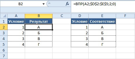
The essence of the approach is to create a “directory” of matching the “Searched_value” argument to a specific result, separately from the main array, in which the conditions and the corresponding values are written:
Then, in the working part of the table, the formula is already written with reference to the reference book that was filled out earlier. Those. in the directory in the “D” column, a value is searched from the “A” column, and when a match is found, the value from the “E” column is displayed in the “B” column.
Formula syntax:
Outputting the result to cell B2:
= CDF (A2; $ D $ 2: $ E $ 5; 2; 0)
Result :
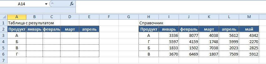
Now imagine a situation where you need to pull the data into one table from another, while the tables are not identical. See example below.
It can be seen that the rows in the columns “Product” of both tables do not match, however, this is not an obstacle to the use of the “CDF” function.
Outputting the result to cell B2:
= CDF ($ A3; $ H $ 3: $ M $ 6; 2; 0)
But when solving, we encounter a new problem - when “pulling” the formula we wrote to the right from column “B” to column “E”, we will have to manually replace the argument “column_number”. This is a laborious and ungrateful business, because another function, COLUMN, comes to the rescue.
Function syntax:
COLUMN ([link])
- Reference is the cell or range of cells for which you want to return a column number.
If you use an entry like:
= COLUMN ()
then the function will display the number of the current column (in the cell of which the formula is written).
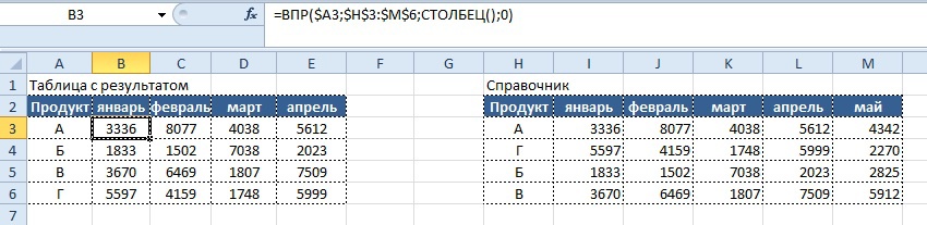
The result is a number that can be used in the “CDF” function, which we will use and get the following formula entry:
Outputting the result to cell B2:
= CDF ($ A3; $ H $ 3: $ M $ 6; COLUMN (); 0)
The COLUMN function determines the number of the current column that will be used by the column_number argument to determine the number of the search column in the directory.
In addition, you can use the design:
= COLUMN () - 1
Instead of the number “1”, you can use any number (and not only subtract it, but also add it to the value obtained) to get the desired result if you don’t want to refer to a specific cell in the column with the number we need.
The result is:
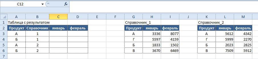
We continue to develop the topic and complicate the condition: imagine that we have two directories with different data on products and it is necessary to display in the table with the result values depending on what type of directory is specified in the column "Reference"
Condition:
- If the column “Reference” indicates the number 1, the data should drag from the table “Reference book_1”, if the number is 2, then from the table “Reference book_2” in accordance with the specified month
The solution that immediately comes to mind is:
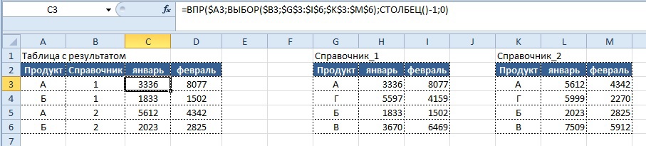
Displaying the result in cell C3:
= IF ($ B3 = 1; CDF ($ A3; $ G $ 3: $ I $ 6; COLUMN () - 1; 0); CDF ($ A3; $ K $ 3: $ M $ 6; COLUMN () - 1; 0 ))
Pros : the name of the directory can be any (text, numbers, and their combination), cons - not very good if there are more than 3 options.
If directory numbers are always numbers, it makes sense to use the following solution:
Displaying the result in cell C3:
= CDF ($ A3; SELECT ($ B3; $ G $ 3: $ I $ 6; $ K $ 3: $ M $ 6); COLUMN () - 1; 0)
Pros : the formula can include up to 254 reference books, minuses - their name must be strictly numeric.
Result for the formula using the “SELECT” function:
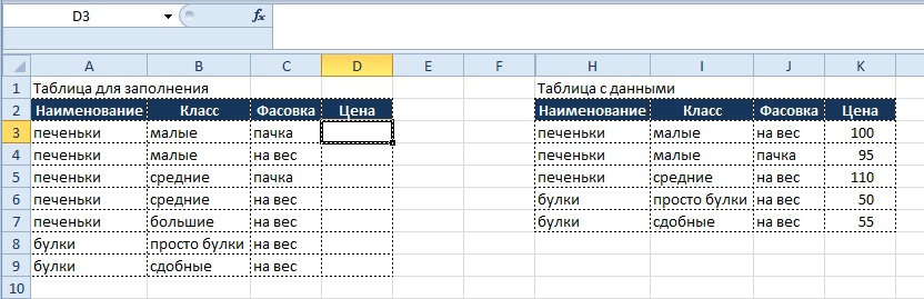
Bonus: CDF on two or more signs in the argument "is_value".
Condition:
- Imagine that, as always, we have an array of data in a tabular form (if not, we bring data to it), from an array on certain grounds it is necessary to get the values and put them into another tabular form.
Both tables are shown below:
As can be seen from the tabular forms, each position has not only the name (which is not unique), but also belongs to a certain class and has its own packaging option.
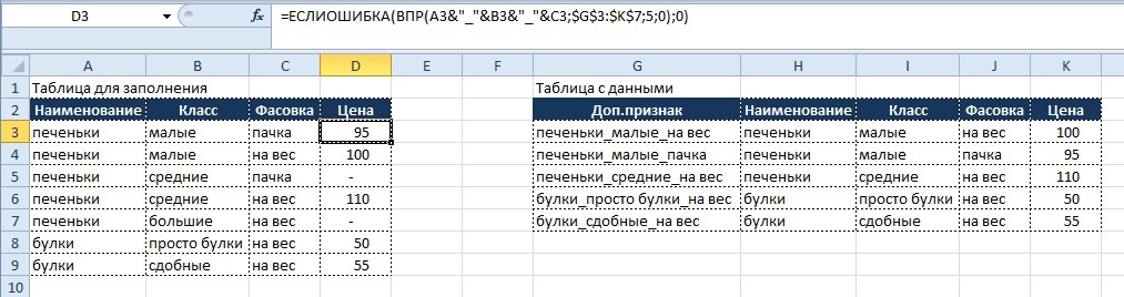
Using a combination of name and class and packing, we can create a new sign, for this in the table with data we create an additional column “Additional attribute”, which we fill in using the following formula:
= H3 & "_" & I3 & "_" & J3
Using the “&” symbol, we combine three signs into one (the separator between words can be any, as well as not be at all, the main thing is to use a similar rule for searching)
The analogue of the formula can be the function "CONCATENATE", in this case it will look like this:
= CLUTCH (H3; "_"; I3; "_"; J3)
After the additional attribute is created for each record in the table with data, we start writing the search function for this attribute, which will look like:
Displaying the result in cell D3:
= ERROR (RR (A2 & "_" & B2 & "_" & C2; $ G $ 2: $ K $ 6; 5; 0); 0)
In the function “CDF”, we use the same combination of three attributes (name_class_packing) as the “search_value” argument, but take it in the table to fill it and enter it directly into the argument (alternatively, we could select the value for the argument in an additional column in table for filling, but this action will be redundant).
I remind you that the use of the IFERROR function (IFERROR) is necessary if the desired value is not found, and the CDF function will display the meaning of "# N / A" (see below).
The result in the picture below:
This technique can be used for more signs, the only condition is the uniqueness of the resulting combinations, if it is not respected, the result will be incorrect.
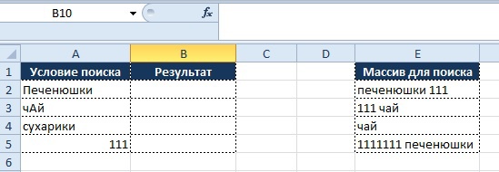
Case_3 Search for a value in an array, or when CDF is unable to help us
Consider the situation when it is necessary to understand whether there are necessary values in the array of cells.
Task:
- in the column “Search condition” the value is indicated and it is necessary to determine whether it is present in the column “Array for search”
Visually, everything looks like this:
As we can see, the “CDF” function is powerless here, since we are not looking for an exact match, but the presence of the desired value in the cell.
To solve the problem, it is necessary to use a combination of several functions, namely:
"IF A"
"ERROR"
"LINE"
"TO FIND"
In order of all, "IF" we have already disassembled earlier, because we move on to the function "ERROR" (IFERROR)
ERROR (value, error_value)
- Value is an argument checked for errors.
- Error_value is the value returned by an error in the calculation using the formula. The following types of errors are possible: # N / A, # VALUE! # REFERENCE! # DEL / 0! # NUMBER! # NAME? and # NULL !.
Important: this formula is almost always required when working with arrays of information and reference books, because it is often the case that the sought value is not in the directory and in this case the function returns an error. If an error is displayed in the cell and the cell participates, for example, in the calculation, then it will also happen with an error. Plus, cells where the formula returned an error can be assigned different values, which facilitate their statistical processing. Also, in the event of an error, you can perform other functions, which is very convenient when working with arrays and allows you to build formulas taking into account fairly extensive conditions.
"LOWER" (LOWER)
LOWER (text)
- Text is text that converts to lower case.
Important: the function "LINE" does not replace characters that are not letters.
The role in the formula: since the FIND function (FIND) searches for and takes into account the case of the text, it is necessary to bring all the text to one register, otherwise the tea will not equal tea, etc. This is relevant if the register value is not a condition for searching and selecting values; otherwise, the “LINE” formula can be omitted, so the search will be more accurate.
Now more about the syntax of the function "FIND" (FIND).
FIND (search_text, view_text, [start_position])
- Searched_text is the text to be found.
- Scanned_text is the text in which you want to find the search text.
- Start_position is the character from which to start the search. The first character in the text "view_text" has the number 1. If the number is not specified, it is considered equal to 1 by default.
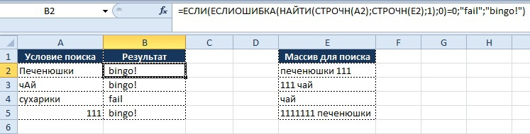
The syntax of the formula-solution will be:
Outputting the result to cell B2:
= IF (ERROR (FIND (LABEL (A2); LOWER (E2); 1); 0) = 0; “fail”; “bingo!”)
Let us analyze the logic of the formula for the actions:
- LINE (A2) - converts the “Searchable_text” argument in a cell in A2 into text with lower case
- The "FIND" function starts searching for the transformed "Search_text" argument in the "View_text" array, which is converted by the "LITTLE (E2)" function, also to text with lower case.
- If the function finds a match, i.e. returns the ordinal number of the first character of the matching word / value, the TRUE condition is triggered in the formula "IF", because the value obtained is not zero. As a result, the Bingo! Value will be displayed in the Result column.
- If the function does not match, i.e. the ordinal number of the first character of the matching word / value is not indicated, and instead of the value, an error is returned, the condition embedded in the formula “ERROR ERROR” is triggered and the value is returned equal to “0”, which corresponds to the FALSE condition in the formula “IF”, since the resulting value is "0". As a result, the value “fail” will be displayed in the Result column.
As can be seen from the figure above, thanks to the "LINE" and "FIND" functions, we find the desired values regardless of the case of the characters and the location in the cell, but it is necessary to pay attention to line 5.
The search condition is set as “111”, but the search array has the value “1111111 cookies”, but the formula gives the result “Bingo!”. This is because the value "111" is included in the series of values "1111111", as a result there is a match. In the opposite case, this condition will not work.
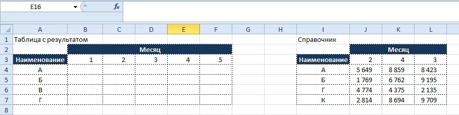
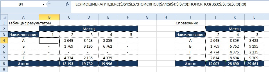
Case_4 Search for a value in an array on several conditions, or when CDF is all the more unable to help us
, « » «» , «» «».
:
:
- «» «».
«» «»
«» (INDEX)
(, _, [_])
- — , .
- , «_» «_» .
- , «_» «_» , «» , «».
- _ — , .
- _ — , .
«» , , «_» «_».
«» (MATCH)
(_, _, [_])
- The desired value is a value that is matched with the values in the argument of the watched array. The search-value argument can be a value (number, text, or logical value) or a reference to a cell containing such a value.
- Scanned_array is the range of cells in which the search is performed.
- Match_type is an optional argument. The number is -1, 0 or 1.
The FIND function searches for the specified element in a range of cells and returns the relative position of that element in the range.
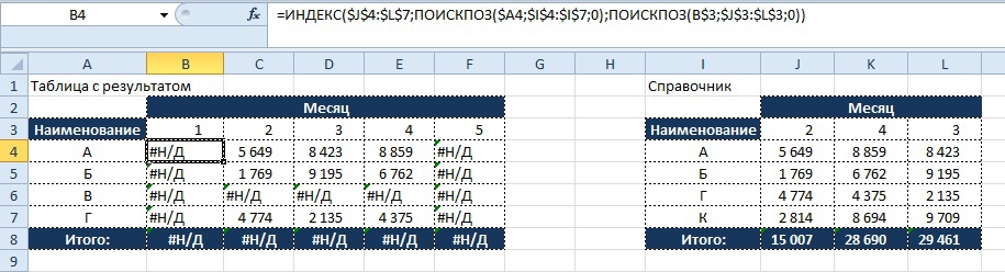
The essence of the use of the combination of the functions "INDEX" and "MATCH" in fact, we search for the coordinates of values by their name on the "coordinate axes".
The Y axis will be the “Name” column, and the X axis will be the “Months” row.
part of the formula:
MATCH ($ A4; $ I $ 4: $ I $ 7; 0)Y, 1, .. «» «1» .
:
(B$3;$J$3:$L$3;0)#/, .. «1» .
, (1; #/) «» «».
B4 :
=($J$4:$L$7; ($A4;$I$4:$I$7;0); (B$3;$J$3:$L$3;0))
, , :
=($J$4:$L$7;1;#/))
, «_» «#/», «B4» .
, «#/», .
Result:
«», , , «0», :
B4:
=(($J$4:$L$7; ($A4;$I$4:$I$7;0); (B$3;$J$3:$L$3;0));0)
:
, «#/» .
_5
, , .
:
- 0 1000 =
- 1001 1500 =
- 1501 2000 =
- 2001 2500 =
- 2501 =
(LOOKUP) , . : .
(_; _; [_])
- _ — , . _ , , , .
- _ — , . _ , .
- _ : ..., -2, -1, 0, 1, 2, ..., AZ, , ; . .
- _ — , . _ , _.
B3:
=(E3;$A$3:$A$7;$B$3:$B$7)
«_» «_» – Excel.
:
B3:
=(E3;{0;1001;1501;2001;2501};{«»;«»;«»;«»;«»})
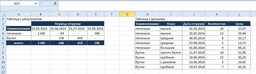
_6
:
(SUMIF) –
(SUMIFS) –
(SUMPRODUCT) –
«» (SUM) , «» :
({=(()*())}
«»
«»:
(1, [2], [3],...)
- 1 — , , .
- 2, 3… — 2 255 , , .
:
- :
, , , .
, «» .
B4:
=(($A4=$H$3:$H$11)*($K$3:$K$11>=B$3)*($K$3:$K$11<C$3);($M$3:$M$11)*($L$3:$L$11))
:
($A4=$H$3:$H$11)– «» «»
($K$3:$K$11>=B$3)*($K$3:$K$11<C$3)– , , . – , – .
($M$3:$M$11)*($L$3:$L$11)– «» «» .
, , .
Result:
, «» «» «», «» , « »:
B4:
=(($A4=$H$3:$H$11)*($J$3:$J$11>=B$3)*($J$3:$J$11<C$3)*(($I$3:$I$11=«»)+($I$3:$I$11=«»));($L$3:$L$11*$K$3:$K$11))
:
(($I$3:$I$11=«»)+($I$3:$I$11=«»))– , «+» .
:
=(($A5=$H$3:$H$11)*($J$3:$J$11>=B$3)*($J$3:$J$11<C$3)*($I$3:$I$11<>« »);($L$3:$L$11)*($K$3:$K$11))
:
($I$3:$I$11<>« »)– , , , , , – « » «<>».
, / , , , , .
Result:
, , , - , ( ).
, - Excel, , !
!
Source: https://habr.com/ru/post/238553/
All Articles