Statistical verification of randomness of binary sequences using NIST methods

Anyone who, in one way or another, has come across cryptography, knows that you cannot do without random number generators. One of the possible applications of such generators, for example, is the generation of keys. But not everyone thinks at the same time, but how “good” a particular generator is. And if he thought about it, he came across the fact that there is no single “official” set of criteria in the world that would assess how much random number data is applicable for this particular field of cryptography. If a sequence of random numbers is predictable, then even the strongest encryption algorithm in which this sequence will be used turns out to be vulnerable — for example, the space of possible keys that an attacker needs to “bite” to get some information, through which he can “crack” »The whole system. Fortunately, various organizations are still trying to bring order here, in particular, the American Institute for Standards NIST has developed a set of tests to assess the randomness of a sequence of numbers. About them will be discussed in this article. But first - a bit of theory (I will try to explain not boring).


')

Random binary sequences

First, by random number generation is meant to obtain a sequence of binary characters 0 and 1, and not bytes, no matter how much the programmers would like. An ideal similar generator is to toss a “perfect” coin (a flat coin with equal probabilities of each side), which would be thrown as many times as necessary, but the problem is that there is nothing ideal, and the performance of such a generator would leave the best (one grown up coin = one bit). Nevertheless, all the tests described below assess how much the random number generator under study “looks like” or “does not look like” on an imaginary ideal coin (not in the rate of receiving “random” signs, but their “quality”).

Secondly, all random number generators are divided into 2 types — truly random — physical random number generators / sensors (DSSH / FDSCH) and pseudo-random — software sensors / random number generators (PDDSH). The first take on the input some random endless process, and on the output they give an infinite (depending on the observation time) sequence 0 and 1. The second ones represent the deterministic function set by the developer, which is initialized by the so-called. grain, after which the output also produces the sequence 0 and 1. Knowing this grain, you can predict the entire sequence. A good PDRCh is one for which it is impossible to predict subsequent values, having the entire history of previous values, having no grain. This property is called direct unpredictability. There is also the reverse unpredictability - the inability to calculate the grain, knowing any number of generated values.

It would seem the easiest way to take truly random / physical RNTS and not think about any predictability. However, there are problems:

• A random phenomenon / process that is taken as a basis may not be able to produce numbers at the desired speed. If you remember the last time you generated a pair of 2048bit keys, then do not flatter yourself. Does this happen very rarely? Then imagine yourself a server accepting hundreds of requests for SSL connections per second (SSL handshake involves generating a pair of random numbers).
• In appearance, random phenomena may not be as random as they would seem. For example, electromagnetic noise can be a superposition of several more or less uniform periodic signals.

Each of the tests offered by NIST receives the final sequence as input. Further, the statistics characterizing a certain property of a given sequence is calculated — it can be a single value or a set of values. After that, these statistics are compared with the standard statistics, which will give a perfectly random sequence. Reference statistics are derived mathematically, many theorems and scientific papers are devoted to this. At the end of the article will be given all references to the sources where the necessary formulas are displayed.

Zero and Alternative Hypotheses

The test is based on the concept of the null hypothesis . I'll try to explain what it is. Suppose we have gathered some statistical information. For example, let it be the number of people who develop lung cancer in a group of 1000 people. And let it be known that some people from this group are smokers, and others are not, and it is known which ones are specific. The next task is to understand whether there is a relationship between smoking and disease. The null hypothesis is the assumption that there is no relationship between the two facts. In our example, this is the assumption that smoking does not cause lung cancer. There is also an alternative hypothesis , which refutes the null hypothesis: i.e. there is a relationship between the phenomena (smoking causes lung cancer). If we proceed to the terms of random numbers, then the null hypothesis is the assumption that the sequence is truly random (the signs of which appear equiprobable and independent of each other). Consequently, if the null hypothesis is true, then our generator produces fairly “good” random numbers.

How is the hypothesis tested? On the one hand, we have statistics calculated on the basis of actually collected data (i.e., by measured sequence). On the other hand, there is a standard statistics obtained by mathematical methods (theoretically calculated), which would have had a truly random sequence. It is obvious that the collected statistics cannot be equal to the standard one - no matter how good our generator is, it is still not perfect. Therefore, a certain error is introduced, for example, 5%. It means that if, for example, the collected statistics deviates from the reference one by more than 5%, then it is concluded that the null hypothesis is not true with high reliability .

Since we are dealing with hypotheses, there are 4 options for the development of events:

1. It is concluded that the sequence is random, and this is the correct conclusion.
2. It is concluded that the sequence is not random, although it was in fact random. Such errors are called errors of the first kind.
3. The sequence is recognized as random, although in fact it is not. Such errors are called errors of the second kind.
4. Sequence rightly rejected

The probability of an error of the first kind is called the level of statistical significance and is designated as α. Those. α is the probability of rejecting a “good” random sequence. This value is determined by the application. In cryptography, α is taken from 0.001 to 0.01.

In each test is calculated so-called. P-value : this is the probability that the experimental generator will produce a sequence no worse than the hypothetical true one. If P value = 1, then our sequence is ideally random, and if it = 0, then the sequence is completely predictable. Further, the P-value is compared with α, and if it is greater than α, then the null hypothesis is accepted and the sequence is considered random. Otherwise, it is rejected.

In tests, α = 0.01 is taken. It follows that:

• If the P-value is ≥ 0.01, the sequence is considered random with a confidence level of 99%.
• If the P-value is <0.01, the sequence is rejected with a confidence level of 99%.

So, we proceed directly to the tests.

Bitwise Frequency Test

Obviously, the more random the sequence, the closer this ratio to 1. This test evaluates how close this ratio is to 1.

We accept each “1” for +1, and each “0” for -1, and count the sum of the entire sequence. This can be written as:
S _n = X ₁ + X ₂ +… + X _n , where X _i = 2x _i - 1.
By the way, it is said that the distribution of the number of “successes” in a series of experiments, where success or failure with a given probability is possible in each experiment, has a binomial distribution.

Take the following sequence: 1011010101

Then S = 1 + (-1) + 1 + 1 + (-1) + 1 + (-1) + 1 + (-1) + 1 = 2

Calculate statistics:


We calculate the P-value through the additional error function :


The complementary error function is defined as:


We see that the result is> 0.01, which means our sequence passed the test. It is recommended to test sequences with a length of at least 100 bits.

Frequency block test

This test is made on the basis of the previous one, only now the values ​​of the proportion "1" / "0" for each block are analyzed by the chi-square method. It is clear that this ratio should be approximately equal to 1.

For example, let the sequence be given 0110011010. Divide it into blocks of 3 bits each (“ownerless” 0 at the end is dropped):
011 001 101

We calculate the proportions π _i for each block: π ₁ = 2/3, π ₂ = 1/3, π ₃ = 1/3. Next, we calculate statistics using the Chi-square method with N degrees of freedom (here N is the number of blocks):


We calculate the P-value through a special function Q :


Q is so-called. incomplete upper gamma function , defined as:


At the same time, function G is the standard gamma function:


A sequence is considered random if the P-value is> 0.01. It is recommended to analyze sequences with a length of at least 100 bits, and the relations M> = 20, M> 0.01n, and N <100 should also be satisfied.

Test for the same consecutive bits

The test searches for all sequences of the same bits, and then analyzes how the number and size of these sequences correspond to the number and size of a truly random sequence. The point is that if a change of 0 to 1 (and vice versa) occurs too rarely, then such a sequence “does not pull” on a random one.

Let the sequence be 1001101011. First, we calculate the proportion of units in the total mass:


Further condition is checked:


If it is not satisfied, then the whole test is considered unsuccessful and that’s the end of it. In our case, 0.63246> 0.1, which means we go further.

Calculate the total number of sign-changing V:


Where if a , or otherwise.



We calculate the P-value through the error function:


If the result is> = 0.01 (as in our example), the sequence is considered random.

Test for the longest sequence of units in a block

The initial sequence of n bits is divided into N blocks, each by M bits, after which each block is searched for the longest sequence of ones, and then it is estimated how close the indicator is to the same indicator for a truly random sequence. Obviously, a similar test for zeros is not required, since if the units are well distributed, then the zeros will also be well distributed.

What is the length of the block? NIST recommends several reference values, how to break into blocks:

Total length, n	Block length, M
128	eight
6272	128
750000	10,000

Let the sequence be given:
11001100 00010101 01101100 01001100 11100000 00000010
01001101 01010001 00010011 11010110 10000000 11010111
11001100 11100110 11011000 10110010

We divide it into blocks of 8 bits (M = 8), then we calculate the maximum sequence of units for each block:

Block	Unit length
11001100	2
00010101	one
01101100	2
01001100	2
11100000	3
00000010	one
01001101	2
01010001	one
00010011	2
11010110	2
10,000,000	one
11010111	3
11001100	2
11100110	3
11011000	2
10110010	2

Next, we consider statistics for different lengths based on the following table:

v i	M = 8	M = 128	M = 10,000
v 0	≤1	& le4	& le10
v 1	2	five	eleven
v 2	3	6	12
v 3	≥4	7	13
v 4		eight	14
v 5		≥9	15
v 6			≥16

How to use this table: we have M = 8, therefore we are looking at only one corresponding column. Consider v _i :
v ₀ = { number of blocks with max. length ≤ 1 } = 4
v ₁ = { number of blocks with max. length = 2 } = 9
v ₂ = { number of blocks with max. length = 3 } = 3
v ₃ = { number of blocks with max. length ≥ 4 } = 0

Calculate the chi-square:


Where the values ​​of K and R are taken from this table:

M	K	R
eight	3	sixteen
128	five	49
10,000	6	75

Theoretical probabilities π _i are given by constants. For example, for K = 3 and M = 8, it is recommended to take π ₀ = 0.2148, π ₁ = 0.3672, π ₂ = 0.2305, π ₃ = 0.1875. (Values ​​for other K and M are given in [2]).


Next, we calculate the P-value:


If it is> 0.01, as in our example, then the sequence is considered to be quite random.

Test of binary matrices

The test analyzes the matrices that are composed of the original sequence, namely, it calculates the ranks of disjoint submatrices constructed from the initial binary sequence. The test is based on Kovalenko’s research [6], where the scientist investigated random matrices consisting of 0 and 1. He showed that it is possible to predict the probabilities that the matrix M x Q will have the rank R, where R = 0, 1, 2 ... min (M, Q). These probabilities are equal:



NIST recommends taking M = Q = 32, as well as the sequence length n = M ^ 2 * N. But for example we take M = Q = 3. Next, we need the probabilities P _M , P _M-1 and P _M-2 . With a small degree of error, the formula can be simplified, and then these probabilities are equal:









So, let the sequence 01011001001010101101 be given. "We decompose" it by matrices - enough for 2 matrices:


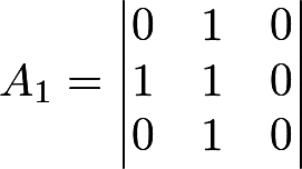
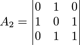
We determine the rank of the matrices: it turns out R ₁ = 2, R ₂ = 3. For the test you need 3 numbers:

• F _M = { number of matrices with rank M } = { number of matrices with rank 3 } = 1
• F _M-1 = 1 (similarly)
• N - F _M - F _M-1 = 2 - 1 - 1 = 0

Calculate the chi-square:


Calculate p-value:


If the result is> 0.01, the sequence is considered random. NIST recommends that the total sequence length be> = 38MQ.

Spectral test

The experimental sequence is considered as a discrete signal for which spectral decomposition is performed in order to identify frequency peaks. Obviously, such peaks will indicate the presence of periodic components, which is not gut. In short, the test reveals peaks exceeding the 95% barrier, after which it checks whether the proportion of these peaks does not exceed 5%.

As you might guess, to represent the sequence as a sum of periodic components, we will use the discrete Fourier transform. It looks like this:


Here x _k is the initial sequence, in which 1 corresponds to +1, and -1 to zero, X _j - the obtained values ​​of the complex amplitudes (complex means that they contain both the real value of the amplitude and the phase).

You ask, where is the periodicity here? The answer is that the exponent can be expressed in terms of trigonometric functions:


For our test, it is not the phases that are interesting, but the absolute values ​​of the amplitudes. And if we calculate these absolute values, then it turns out that they are symmetric (this is a well-known fact when moving from complex to real values), so for further consideration we will take only half of these values ​​(from 0 to n / 2) - the rest do not carry additional information.

Let us show all this with an example. Let the sequence be 1001010011.
Then x = {1, -1, -1, 1, -1, 1, -1, -1, 1, 1}.

Here's how Fourier decomposition can be done, for example, in the GNU Octave program:

octave:1> x = [1, -1, -1, 1, -1, 1, -1, -1, 1, 1] x = 1 -1 -1 1 -1 1 -1 -1 1 1 octave:2> abs(fft(x)) ans = 0.0000 2.0000 4.4721 2.0000 4.4721 2.0000 4.4721 2.0000 4.4721 2.0000 

We see that there is symmetry. Therefore, five values ​​are enough for us: 0, 2, 4.4721, 2, 4.4721.

Next, we calculate the boundary value by the formula


It means that if the sequence is truly random, then 95% of the peaks should not exceed this limit.

Calculate the maximum number of peaks, which must be less than T:


Next, we look at the result of the decomposition and see that all our 4 peaks are less than the boundary value. Further we estimate this difference:


Calculate p-value:


It turned out> 0.01, so the hypothesis of randomness is accepted. And yes, for the test it is recommended to take at least 1000 bits.

Test for non-intersecting patterns

The experimental sequence is divided into blocks of the same length. For example:
1010010010 1110010110

In each block we will look for some pattern, for example, “001”. The word disjoint means that if a pattern is found within a sequence, the following comparison will not capture a single bit of the pattern found. As a result of the search for each i-th block will be found the number of W _i equal to the number of cases found.

So, for our blocks, W ₁ = 2 and W ₂ = 1:
101 001 001 0
111 001 0110

We calculate the expectation and variance, as if our sequence was truly random. Below are the formulas. Here N = 2 (number of blocks), M = 10 (block length), m = 3 (sample length).





Calculate the chi-square:



Calculate the final P-value through an incomplete gamma function:



We see that the P-value is> 0.1, which means that the sequence is quite random.

We only rated one template. In fact, you need to check all the combinations of templates, and besides, for different lengths of these templates. How much is needed is determined on the basis of specific requirements, but usually m takes 9 or 10. To get meaningful results, you should take N <100 and M> 0.01 * n.

Test for intersecting patterns

This test differs from the previous one in that when the search pattern is found, the search window shifts not by the pattern length, but only by 1 bit. In order not to clutter the article, we will not give an example of calculation by this method. It is completely analogous.

Mauer Universal Test

The test assesses how far away the patterns within the sequence are from each other. The meaning of the test is to understand how the sequence is compressible (of course, I mean lossless compression). The more compressible the sequence, the less random it is. The algorithm of this test is very cumbersome for the Habra-format, so we omit it.

Linear complexity test

The test is based on the assumption that the experimental sequence was obtained through a linear feedback shift register (or LFSR, Linear feedback shift register). This is a well-known method of obtaining an infinite sequence: here each next bit is obtained as a certain function of the bits "sitting" in the register. The minus of the LFSR is that it always has a finite period, i.e. the sequence will be repeated sooner or later. The greater the length of the LFSR, the better the random sequence.

The initial sequence is divided into equal blocks of length M. Further, for each block using the Berlekamp – Massey algorithm [10], its linear complexity (L _i ) is found, i.e. length lfsr. Then for all found L _i , the Chi-square distribution with 6 degrees of freedom is estimated. We show by example.

Let block 1101011110001 (M = 13) be given, for which the Berlekamp – Massey algorithm issued L = 4. Make sure that this is so. Indeed, it is not difficult to guess that for this block each next bit is obtained as the sum (modulo 2) of the 1st and 2nd bits (numbering from 1):
x ₅ = x ₁ + x ₂ = 1 + 1 = 0
x ₆ = x ₂ + x ₃ = 1 + 0 = 1
x ₇ = x ₃ + x ₄ = 1 + 0 = 1
etc.

Calculate the expectation of the formula


For each block, we calculate the value of T _i :


Further, on the basis of the set T, we calculate the set v ₀ , ..., v ₆ in the following way:

• if T _i <= -2.5, then v ₀ ++
• if -2.5 <T _i <= -1.5, then v ₁ ++
• if -1.5 <T _i <= -0.5, then v ₂ ++
• if -0.5 <T _i <= 0.5, then v ₃ ++
• if 0.5 <T _i <= 1.5, then v ₄ ++
• if 1.5 <T _i <= 2.5, then v ₅ ++
• if T _i > 2.5, then v ₆ ++

We have 7 possible outcomes, and therefore we calculate Chi-square with the number of degrees of freedom 7 - 1 = 6:

The probabilities π _i in the test are rigidly set and equal, respectively: 0.010417, 0.03125, 0.125, 0.5, 0.25, 0.0625, 0.020833. (π _i for a larger number of degrees of freedom can be calculated by the formulas given in [2]).

Calculate p-value:


If the result is> 0.01, the sequence is considered random. For real tests, it is recommended to take n> = 10 ^ 6 and M in the range from 500 to 5000.

Subsequence test

The frequency of finding all possible sequences of length “m” bits within the original sequence is analyzed. In addition, each sample is searched independently, i.e. It is possible, as it were, to “superimpose” one found sample on another. Obviously, the number of all possible samples will be 2 ^m . If the sequence is large enough and random, then the probability of finding each of these samples is the same. (By the way, if m = 1, then this test "degenerates" into the already described test for the ratio of "0" or "1").

The basis of the test is the work [8] and [11]. It describes 2 indicators (∇ψ ² _m and ∇ ^{2 2} _m ), which characterize how much the frequency of appearance of samples correspond to the same frequencies for a truly random sequence. We show the algorithm by example.

Let sequence 0011011101 be given with length n = 10 and also m = 3.

First, 3 new sequences are formed, each of which is obtained by adding m-1 first bits of the sequence to its end. It turns out:

• For m = 3: 0011011101 00 (added 2 bits to the end)
• For m-1 = 2: 0011011101 0 (added 1 bit to the end)
• For m-2 = 1: 0011011101 (source sequence)

Next we find the frequency of occurrence of all blocks of length m, m-1 and m-2, respectively:

• v ₀₀₀ = 0, v ₀₀₁ = 1, v ₀₁₀ = 1, v ₀₁₁ = 2, v ₁₀₀ = 1, v ₁₀₁ = 2, v ₁₁₀ = 2, v ₁₁₁ = 0
• v ₀₀ = 1, v ₀₁ = 3, v ₁₀ = 3, v ₁₁ = 3
• v ₀ = 4, v ₁ = 6

We calculate the necessary statistics by the formulas:


Substitute:


Then:





Totals:


So, both P-values ​​are> 0.01, which means the sequence is considered random.

Approximate entropy

The method of approximate entropy (Approximate Entropy) initially manifested itself in medicine, especially in cardiology. In general, according to the classical definition, entropy is a measure of chaos: the higher it is, the more unpredictable phenomena. Good or bad depends on the context. For random sequences used in cryptography, it is important to have high entropy - this means that it will be difficult to predict subsequent random bits based on what we already have. But, for example, if we take the heart rate measured with a given period as a random variable, the situation is different: there are many studies (for example, [12]) that prove that the lower the heart rate variability, the less likely the likelihood of heart attacks and other unpleasant phenomena . It is obvious that a person’s heart cannot beat with a constant frequency. However, some die from heart attacks, while others do not. Therefore, the method of approximate entropy allows us to estimate how seemingly random phenomena really are random .

Specifically, the test calculates the frequency of occurrence of various samples of a given length (m), and then similar frequencies, but already for samples of length m + 1. The frequency distribution is then compared to the reference Chi-squared distribution. As in the previous test, the samples may overlap.

We show by example. Let the sequence 0100110101 (length n = 10) be given, and take m = 3.

To begin with, we complement the sequence with the first m-1 bits. It turns out 0100110101 01.

Calculate the occurrence of each of the 8 different blocks. It turns out:
k ₀₀₀ = 0, k ₀₀₁ = 1, k ₀₁₀ = 3, k ₀₁₁ = 1, k ₁₀₀ = 1, k ₁₀₁ = 3, k ₁₁₀ = 1, k ₁₁₁ = 0.

Calculate the corresponding frequencies according to the formula C _i ^m = k _i / n:
C ₀₀₀ ³ = 0, C ₀₀₁ ³ = 0.1, C ₀₁₀ ³ = 0.3, C ₀₁₁ ³ = 0.1, C ₁₀₀ ³ = 0.1, C ₁₀₁ ³ = 0.3, C ₁₁₀ ³ = 0.1, C ₁₁₁ ³ = 0.

Similarly, we assume the frequency of occurrence of sub-blocks of length m + 1 = 4. There are already 2 ⁴ = 16:
C ₀₀₁₁ ⁴ = C ₀₁₀₀ ⁴ = C ₀₁₁₀ ⁴ = C ₁₀₀₁ ⁴ = C ₁₁₀₁ ⁴ = 0.1, C ₀₁₀₁ ⁴ = 0.2, C ₁₀₁₀ ⁴ = 0.3. Remaining frequencies = 0.

Calculate φ ³ and φ ⁴ (note that the natural logarithm is here):





Calculate the chi-square:


P-value:


The resulting value is> 0.01, which means the sequence is considered random.

Cumulative test

We take each zero bit of the original sequence for -1, and each one - for +1, after which we calculate the sum. Intuitively, the more random the sequence, the faster this amount will tend to zero. On the other hand, imagine that a sequence is given, consisting of 100 zeros and 100 units, running in a row: 00000 ... 001111 ... 11. Here, the amount will be equal to 0, but it is obvious that to call such a sequence a random "hand will not rise." Therefore, a deeper criterion is needed. And this criterion is partial amounts. We will gradually calculate the amounts starting from the first element:
S ₁ = x ₁
S ₂ = x ₁ + x ₂ S ₃ = x ₁ + x ₂ + x ₃ ...
S _n = x ₁ + x ₂ + x ₃ +… + x _n

Next is the number z = maximum among these sums.

Finally, the P-value is calculated according to the following formula (see its derivation in [9]):


Where:




Here Φ is the distribution function of the standard normal random variable. We recall that the standard normal distribution is the well-known Gaussian distribution (in the shape of a bell), whose expectation is 0 and variance 1. It looks like this:


If the resulting P-value> 0.01, then the sequence is considered random.

By the way, this test has 2 modes: the first one we just reviewed, and the second amount is calculated starting from the last element.

Random deviation test

This test is similar to the previous one: in a similar way, partial sums of a normalized sequence (ie, consisting of -1 and 1) are considered. Let sequence 0110110101 be given and let S (i) be the partial sum from 1 to the i-th element. Put these points on the graph, preliminarily adding “0” to the beginning and end of the sequence S (i) - this is necessary for the integrity of the further calculations:

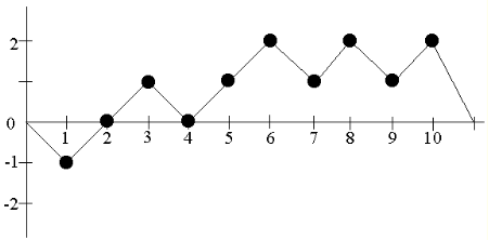
Note the points where the graph intersects the horizontal axis - these points will divide the sequence into so-called. cycles . Here we have 3 cycles: {0, -1, 0}, {0, 1, 0} and {0, 1, 2, 1, 2, 1, 2, 0}. Further, it is said that each of these cycles successively takes on different states . For example, the first cycle 2 times takes the state "0" and 1 time the state "-1". For this test, the states from -4 to 4 are of interest. Add all the occupations in these states to the following table:

State (x)	Cycle number 1	Cycle number 2	Cycle number 3
-four	0	0	0
-3	0	0	0
-2	0	0	0
-one	one	0	0
one	0	one	3
2	0	0	3
3	0	0	0
four	0	0	0

On the basis of this table, we form another table: in it horizontally, the number of cycles will go, taking a given state:

State (x)	Never	1 time	2 times	3 times	4 times	5 times
-four	3	0	0	0	0	0
-3	3	0	0	0	0	0
-2	3	0	0	0	0	0
-one	2	one	0	0	0	0
one	one	one	0	one	0	0
2	2	0	0	one	0	0
3	3	0	0	0	0	0
four	3	0	0	0	0	0

Then, for each of the eight states, a Chi-square of statistics is calculated using the formula


Where v _k (x) is the values ​​in the table for a given state, J is the number of cycles (we have 3), π _k (x) are the probabilities that the state “x” will occur k times in a truly random distribution (they are known).

For example, for x = 1 we get:


The values ​​of π for the remaining x are given in [2].

Calculate p-value:


If it is> 0.01, then the conclusion is made about randomness. As a result, it is necessary to calculate 8 P-values. Some may be more than 0.01, some - less. In this case, the final decision on the sequence is made on the basis of other tests.

Variety test for arbitrary deviations

It is almost similar to the previous test, but a wider set of states is taken: -9, -8, -7, -6, -5, -4, -3, -2, -1, +1, +2, +3, + 4, +5, +6, +7, +8, +9. But the main difference is that here the P-value is calculated not through the gamma function (igamc) and Chi-square, but through the error function (erfc). For exact formulas the reader can refer to the original document.

Below is a list of sources that you can see if you want to delve into the topic:

1. csrc.nist.gov/groups/ST/toolkit/rng/stats_tests.html
2. csrc.nist.gov/groups/ST/toolkit/rng/documents/SP800-22rev1a.pdf
3. Central limit theorem
4. Anant P. Godbole and Stavros G. Papastavridis, (ed), Runs and patterns in probability: Selected papers. Dordrecht: Kluwer Academic, 1994
5. Pal Revesz, Random Walk in Random and Non-Random Environments. Singapore: World Scientific, 1990
6. I. N. Kovalenko, Theory of probability and its applications, 1972
7. O. Chrysaphinou, S. Papastavridis, “A Limit Theorem” on the Sequence of Independent Trials. ”Fields, Vol. 79, 1988
8. IJ Good, “The serial test for sampling numbers,” Cambridge, 1953
9. A. Rukhin, “Approximate entropy for testing randomness,” Journal of Applied Probability, 2000
10. Berlekampa - Massey Algorithm
11. DE Knuth, The Art of Computer Programming. Vol. 2 & 3, 1998
12. www.ncbi.nlm.nih.gov/pubmed/8466069