How to deal with repost or a couple of words about perceptual hashes
This publication focuses on perceptual image hashes and their use (for example, searching for duplicates).
Perceptual hash algorithms describe a class of functions for generating comparable hashes. They use various properties of the image to build an individual “print”. In the future, these "prints" can be compared with each other.
If the hashes are different, then the data is different. If the hashes match, then the data is most likely the same (since there is a possibility of collisions, then the same hashes do not guarantee the coincidence of the data). This article focuses on several popular methods for constructing perceptual image hashes, as well as a simple way to deal with collisions. Anyone interested, please under the cat.
There are many different approaches to the formation of perceptual image hashes. All of them are united by 3 main stages:
')
In this publication, we will not deal with the implementation of the above algorithms. It is an overview and tells about different approaches to the construction of hashes.
We will consider 4 different hash algorithms: Simple Hash [4], DCT Based Hash [1], [11], Radial Variance Based Hash [1], [5] and Marr-Hildreth Operator Based Hash [1], [6] .
The essence of this algorithm is to display the average value of low frequencies. In images, high frequencies provide detail, while low ones show structure. Therefore, to build such a hash function, which for similar images will produce a close hash, you need to get rid of high frequencies. Principle of operation:
The resulting hash is resistant to scaling, compressing or stretching the image, changing the brightness, contrast, color manipulation. But the main advantage of the algorithm is its speed. To compare hashes of this type, the function of the normalized Hamming distance is used.
Source image
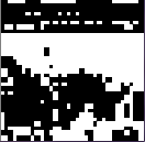
The resulting "imprint"
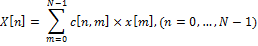
The discrete cosine transform (DCT, DCT) [7] is one of the orthogonal transforms, which is closely related to the discrete Fourier transform (DFT) and is a homomorphism of its vector space. DCT, like any Fourier-oriented transform, expresses a function or signal (a sequence of a finite number of data points) as a sum of sinusoids with different frequencies and amplitudes. DCT uses only cosine functions, in contrast to the DFT, which uses both cosine and sine functions. There are 8 types of DCT [7]. The most common is the second type. We will use it to build a hash function.
Let's see what the second type of DCT is:
Let x [m], where m = 0, ..., N - 1 is the sequence of the signal of length N. We define the second type of DCT as
This expression can be rewritten as:
where c [n, m] is an element of the DCT matrix at the intersection of row n and column m.
DCT matrix is defined as:
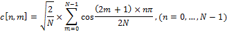
This matrix is very convenient for calculating DCT. DCT can be calculated in advance for any necessary length. Thus, DCT can be represented as:
DCT = M × I × M '
Where M is the DCT matrix, I is the image of a square size, M 'is the inverse matrix.
Low-frequency DCT coefficients are most stable to image manipulation. This is because most of the signal information is usually concentrated in several low frequency coefficients. As a matrix I, an image is usually taken, compressed to a size of 32x32 and simplified using various filters, for example, bleaching. The result is a DCT matrix (I), in the upper left corner of which the low-frequency coefficients are located. To build a hash, the left upper block of frequencies 8x8 is taken. Then a 8 byte hash is built from this block by finding the average and building a chain of bits (as in Simple Based Hash).
Here are the steps to build a hash using this algorithm:
The main advantages of such a hash: resistance to small rotations, blurring and image compression, as well as the speed of comparison of hashes, due to their small size. To compare hashes of this type, the Hamming distance function is used.
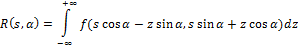
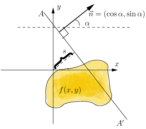
The idea of the Radial Variance Based Hash algorithm is to build a ray dispersion vector (LVD) based on the Radon transform [5]. Then DCT is applied to the LVD and a hash is calculated. The Radon transform is an integral transform of a multi-variable function along a straight line. It is resistant to image processing through various manipulations (for example, compression) and geometric transformations (for example, rotations). In the two-dimensional case, the Radon transform for the function f (x, y) looks like this:
The Radon transform has a simple geometric meaning: it is an integral of the function along a straight line perpendicular to the vector n = (cos a, sin a) and passing at a distance s (measured along the vector n, with the corresponding sign) from the origin.
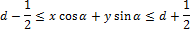
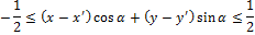
To expand the Radon transform for discrete images, the linear integral along the straight line d = x ∙ cos α + y ∙ sin α can be approximated by summing the values of all pixels lying in a line one pixel wide:
It was later found that it is better to use the variance instead of the sum of the pixel values along the projection line [6]. Dispersion handles brightness discontinuities along the projection line much better. Such brightness discontinuities appear because of edges that are orthogonal to the projection line.
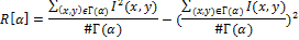
Now we define the ray vector of dispersion. Let Γ (α) be the set of pixels on the projection line corresponding to a given angle. Let (x ′, y ′) be the coordinates of the central pixel in the image. x, y belong to Γ (α) if and only if
Now we define the radial vector variance vector:
Let I (x, y) denote the pixel brightness (x, y), #Γ (α) is the power of the set, then the ray vector of dispersion R [α], where α = 0.1, ..., 179 is defined as
It is enough to construct a vector with 180 angle values, since the Radon transform is symmetric. The resulting vector can be used to build a hash, but this algorithm proposes some other improvement - to apply DCT to the received vector. The result is a vector that inherits all the important properties of DCT. The first 40 coefficients of the obtained vector, which correspond to low frequencies, are taken as a hash. Thus, the size of the resulting hash is 40 bytes.
So, we list the steps for constructing a hash using this algorithm:
For comparison, hashes of this type are used to search for the peak of the mutual correlation function.
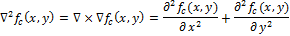
The operator Marra-Hildreta [16] allows you to define the edges on the image. Generally speaking, the border in an image can be defined as an edge or contour that separates adjacent parts of the image, which have relatively different characteristics in accordance with certain features. These features can be color or texture, but the most commonly used is a gray gradation of the image color (brightness). The result of the definition of boundaries is a map of boundaries. The border map describes the classification of borders for each image pixel. If the boundaries are defined as an abrupt change in brightness, then derivatives can be used to find them or a gradient.
Let function denotes the brightness level for the line (one-dimensional array of pixels). The first approach to determining the boundaries is to find the local extrema of the function, that is, the first derivatives. The second approach (the Laplace method) is to find the second derivatives [one].
Both approaches can be adapted for the case of two-dimensional discrete images, but with some problems. To find derivatives in a discrete case, an approximation is required. In addition, noise in the image can significantly impair the process of searching for boundaries. Therefore, before determining the boundaries to the image, you must apply a filter that suppresses noise. To build a hash, you can choose an algorithm that uses the Laplace operator (2 approach) and the Gauss filter.
We define a continuous Laplacian (Laplace operator):
Let be determines the brightness of the image. Then continuous Laplacian is defined as:
Zeroing and there are points corresponding to the boundary of the function , since these are the points at which the second derivative vanishes. Various filters (discrete Laplace operators) can be obtained from continuous Laplacian. Such a filter
  , can be applied to a discrete image by using the convolution of functions. Laplace operator for image
  can be rewritten as:

where * denotes the convolution of functions. To build a boundary map, you need to find the treatment of zero discrete operator .
.
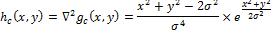
Now consider the Marra-Hildreth operator. It is also called the Laplacian from the Gaussian filter (LoG) - this is a special type of discrete Laplace operator. LoG is constructed by applying the Laplace operator to a Gauss filter (function). The peculiarity of this operator is that it can select borders at a certain scale. Scale variables can be varied in order to better define the boundaries.
The Gauss filter is defined as:

Convolution with Laplace operation can be swapped, because the derivative and convolution are linear operators:

This property allows you to pre-calculate the operator , because it does not depend on the image ( ).
(operator Marra-Hildreta, Laplacian from the Gauss filter, LoG). LoG hc (x, y) is defined as:
To use LoG in discrete form, we will make a discretization of this equation, substituting the desired scale variable. By default, its value is taken as 1.0. The filter can then be applied to the image using discrete convolution.
Define the discrete convolution:
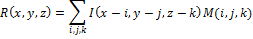
Let x, y, z be the pixel width, length and depth of the image I.
The result of the R convolution of the image I with the mask M is defined as:
Now we list the steps of the algorithm that uses the Marr-Hildret operator to build the hash:
The size of the resulting hash is not small, however, the comparison of two hashes takes a rather short time compared with the Radial algorithm, since the function of the normalized Hamming distance is used. Also, this algorithm is sensitive to image rotation, but is resistant to scaling, dimming, and compression.
Hamming distance determines the number of different positions between two binary sequences.
Definition:
Let A be an alphabet of finite length. - binary sequences (vectors). Hamming distance Δ between x and y is defined as:
This method of comparing hash values is used in the DCT Based Hash method. The hash is 8 bytes in size, so the Hamming distance lies in the [0, 64] segment. The smaller the Δ value, the more similar the images.
To facilitate comparison, the Hamming distance can be normalized using the length of the vectors:
The normalized Hamming distance is used in the Simple Hash and Marr-Hildreth Operator Based Hash algorithms. Hamming distance lies in the interval [0,1] and the closer Δ to 0, the more similar the images.
The correlation between the two signals is defined as:
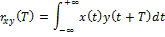
where x (t) and y (t) are two continuous functions of real numbers. The function rxy (t) describes the displacement of these two signals relative to time T. The variable T determines how far the signal is shifted to the left. If the signals x (t) and y (t) are different, the function rxy T is said to be mutually correlated.
Define the Normalized Mutual Correlation Function:
Let xi and yi, where i = 0, ... N - 1 are two sequences of real numbers, and N is the length of both sequences. IAF with delay d will be defined as:
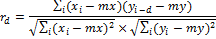
where mx and my denote the average value for the corresponding sequence.
The peak of the mutual correlation function (PCC) is the maximum value of the function rd, which can be achieved on the interval d = 0, N.
PCC is used to compare hash values in the Radial Variance Based Hash algorithm. PCC ∈ [0,1], the greater its value, the more similar the images.
We considered 4 different approaches in the implementation of hash algorithms. The perceptual hashes are wide in scope, from searching for similar images to detecting spam in pictures.
In our project, we use a perceptual hash to identify duplicate images. At the same time, it is often possible to successfully compare among themselves images containing watermarks (obtained from different sources) or images with cropped edges.
Radial Variance Based Hash can be considered the best algorithm for finding duplicates, but it is extremely difficult to use it on large amounts of data, due to the very time-consuming comparison of hashes.
For ourselves, we chose DCT based Hash. We use 64-bit hash, this is quite enough to find duplicates, but such a small hash size inevitably leads to collisions. With collisions, we struggle to construct a histogram (spectrum) for the image.
Each component of the spectrum means the relative number of colors of one or another range in the image, in other words, it shows the distribution of colors in the image. It looks like this:
Thus, we first look for images comparing the hash, and then compare the histograms, if the histograms are significantly different, then such an image is not considered to be similar. The histograms themselves can be compared by counting the cross-correlation as well as by comparing Radial Variance Based Hash using the Pearson cross-correlation:
If this topic is interesting to the community, in the next article I will talk specifically about our implementation of DCT hash, as well as how to find the Hamming distance.
Perceptual hash algorithms describe a class of functions for generating comparable hashes. They use various properties of the image to build an individual “print”. In the future, these "prints" can be compared with each other.
If the hashes are different, then the data is different. If the hashes match, then the data is most likely the same (since there is a possibility of collisions, then the same hashes do not guarantee the coincidence of the data). This article focuses on several popular methods for constructing perceptual image hashes, as well as a simple way to deal with collisions. Anyone interested, please under the cat.
Overview
There are many different approaches to the formation of perceptual image hashes. All of them are united by 3 main stages:
')
- Preliminary processing. At this stage, the image is reduced to a form in which it is easier to process it to build a hash. This may be the use of various filters (for example, Gauss), discoloration, image size reduction, etc.
- Basic calculations. A matrix (or a vector) is constructed from the image obtained at stage 1. The matrix (vector) can be a matrix of frequencies (for example, after a Fourier transform), a histogram of brightness, or an even simpler image.
- Build a hash. From the matrix (vector) obtained in stage 2, some (possibly all) coefficients are taken and converted into a hash. Usually the hash is obtained in size from 8 to ~ 100 bytes. The calculated hash values are then compared using functions that calculate the “distance” between two hashes.
In this publication, we will not deal with the implementation of the above algorithms. It is an overview and tells about different approaches to the construction of hashes.
Perceptual Hash Algorithms
We will consider 4 different hash algorithms: Simple Hash [4], DCT Based Hash [1], [11], Radial Variance Based Hash [1], [5] and Marr-Hildreth Operator Based Hash [1], [6] .
Simple Hash (aka Average Hash)
The essence of this algorithm is to display the average value of low frequencies. In images, high frequencies provide detail, while low ones show structure. Therefore, to build such a hash function, which for similar images will produce a close hash, you need to get rid of high frequencies. Principle of operation:
- Reduce the size. The fastest way to get rid of high frequencies is to reduce the image. The image is reduced to a size in the range of 32x32 and 8x8.
- Remove color. A small image is converted to grayscale, so the hash is reduced three times.
- Calculate the average color value for all pixels.
- Build a chain of bits. For each pixel, a color replacement is made by 1 or 0, depending on whether it is larger or less than the average.
- Build a hash. Translation of 1024 bits into one value. The order does not matter, but usually the bits are written from left to right, top to bottom.
The resulting hash is resistant to scaling, compressing or stretching the image, changing the brightness, contrast, color manipulation. But the main advantage of the algorithm is its speed. To compare hashes of this type, the function of the normalized Hamming distance is used.
Source image
The resulting "imprint"
Discrete Cosine Transform Based Hash (aka pHash)
The discrete cosine transform (DCT, DCT) [7] is one of the orthogonal transforms, which is closely related to the discrete Fourier transform (DFT) and is a homomorphism of its vector space. DCT, like any Fourier-oriented transform, expresses a function or signal (a sequence of a finite number of data points) as a sum of sinusoids with different frequencies and amplitudes. DCT uses only cosine functions, in contrast to the DFT, which uses both cosine and sine functions. There are 8 types of DCT [7]. The most common is the second type. We will use it to build a hash function.
Let's see what the second type of DCT is:
Let x [m], where m = 0, ..., N - 1 is the sequence of the signal of length N. We define the second type of DCT as
This expression can be rewritten as:
where c [n, m] is an element of the DCT matrix at the intersection of row n and column m.
DCT matrix is defined as:
This matrix is very convenient for calculating DCT. DCT can be calculated in advance for any necessary length. Thus, DCT can be represented as:
DCT = M × I × M '
Where M is the DCT matrix, I is the image of a square size, M 'is the inverse matrix.
Low-frequency DCT coefficients are most stable to image manipulation. This is because most of the signal information is usually concentrated in several low frequency coefficients. As a matrix I, an image is usually taken, compressed to a size of 32x32 and simplified using various filters, for example, bleaching. The result is a DCT matrix (I), in the upper left corner of which the low-frequency coefficients are located. To build a hash, the left upper block of frequencies 8x8 is taken. Then a 8 byte hash is built from this block by finding the average and building a chain of bits (as in Simple Based Hash).
Here are the steps to build a hash using this algorithm:
- Remove color. To suppress unnecessary treble;
- Apply a median filter [8] to reduce noise. At the same time, the image is divided into so-called “windows”, then each window is replaced with a median [9] for adjacent windows;
- Reduce image to size 32x32;
- Apply DCT to the image;
- Build a hash.
The main advantages of such a hash: resistance to small rotations, blurring and image compression, as well as the speed of comparison of hashes, due to their small size. To compare hashes of this type, the Hamming distance function is used.
Radial Variance Based Hash
The idea of the Radial Variance Based Hash algorithm is to build a ray dispersion vector (LVD) based on the Radon transform [5]. Then DCT is applied to the LVD and a hash is calculated. The Radon transform is an integral transform of a multi-variable function along a straight line. It is resistant to image processing through various manipulations (for example, compression) and geometric transformations (for example, rotations). In the two-dimensional case, the Radon transform for the function f (x, y) looks like this:
The Radon transform has a simple geometric meaning: it is an integral of the function along a straight line perpendicular to the vector n = (cos a, sin a) and passing at a distance s (measured along the vector n, with the corresponding sign) from the origin.
To expand the Radon transform for discrete images, the linear integral along the straight line d = x ∙ cos α + y ∙ sin α can be approximated by summing the values of all pixels lying in a line one pixel wide:
It was later found that it is better to use the variance instead of the sum of the pixel values along the projection line [6]. Dispersion handles brightness discontinuities along the projection line much better. Such brightness discontinuities appear because of edges that are orthogonal to the projection line.
Now we define the ray vector of dispersion. Let Γ (α) be the set of pixels on the projection line corresponding to a given angle. Let (x ′, y ′) be the coordinates of the central pixel in the image. x, y belong to Γ (α) if and only if
Now we define the radial vector variance vector:
Let I (x, y) denote the pixel brightness (x, y), #Γ (α) is the power of the set, then the ray vector of dispersion R [α], where α = 0.1, ..., 179 is defined as
It is enough to construct a vector with 180 angle values, since the Radon transform is symmetric. The resulting vector can be used to build a hash, but this algorithm proposes some other improvement - to apply DCT to the received vector. The result is a vector that inherits all the important properties of DCT. The first 40 coefficients of the obtained vector, which correspond to low frequencies, are taken as a hash. Thus, the size of the resulting hash is 40 bytes.
So, we list the steps for constructing a hash using this algorithm:
- Remove color to suppress unnecessary treble;
- Blur an image using a Gaussian blur [10]. The image is converted using the Gauss function to suppress some noise;
- Apply gamma correction to eliminate image fading.
- Build the radial vector of the dispersion;
- Apply DCT to the dispersion vector;
- Build a hash.
For comparison, hashes of this type are used to search for the peak of the mutual correlation function.
Marr-Hildreth Operator Based Hash
The operator Marra-Hildreta [16] allows you to define the edges on the image. Generally speaking, the border in an image can be defined as an edge or contour that separates adjacent parts of the image, which have relatively different characteristics in accordance with certain features. These features can be color or texture, but the most commonly used is a gray gradation of the image color (brightness). The result of the definition of boundaries is a map of boundaries. The border map describes the classification of borders for each image pixel. If the boundaries are defined as an abrupt change in brightness, then derivatives can be used to find them or a gradient.
Let function
denotes the brightness level for the line (one-dimensional array of pixels). The first approach to determining the boundaries is to find the local extrema of the function, that is, the first derivatives. The second approach (the Laplace method) is to find the second derivatives [one].Both approaches can be adapted for the case of two-dimensional discrete images, but with some problems. To find derivatives in a discrete case, an approximation is required. In addition, noise in the image can significantly impair the process of searching for boundaries. Therefore, before determining the boundaries to the image, you must apply a filter that suppresses noise. To build a hash, you can choose an algorithm that uses the Laplace operator (2 approach) and the Gauss filter.
We define a continuous Laplacian (Laplace operator):
Let be
determines the brightness of the image. Then continuous Laplacian is defined as:Zeroing
and there are points corresponding to the boundary of the function , since these are the points at which the second derivative vanishes. Various filters (discrete Laplace operators) can be obtained from continuous Laplacian. Such a filter , can be applied to a discrete image by using the convolution of functions. Laplace operator for image can be rewritten as:where * denotes the convolution of functions. To build a boundary map, you need to find the treatment of zero discrete operator
.Now consider the Marra-Hildreth operator. It is also called the Laplacian from the Gaussian filter (LoG) - this is a special type of discrete Laplace operator. LoG is constructed by applying the Laplace operator to a Gauss filter (function). The peculiarity of this operator is that it can select borders at a certain scale. Scale variables can be varied in order to better define the boundaries.
The Gauss filter is defined as:
Convolution with Laplace operation can be swapped, because the derivative and convolution are linear operators:
This property allows you to pre-calculate the operator
, because it does not depend on the image ( ).(operator Marra-Hildreta, Laplacian from the Gauss filter, LoG). LoG hc (x, y) is defined as:
To use LoG in discrete form, we will make a discretization of this equation, substituting the desired scale variable. By default, its value is taken as 1.0. The filter can then be applied to the image using discrete convolution.
Define the discrete convolution:
Let x, y, z be the pixel width, length and depth of the image I.
The result of the R convolution of the image I with the mask M is defined as:
Now we list the steps of the algorithm that uses the Marr-Hildret operator to build the hash:
- Remove color to suppress unnecessary treble;
- Convert image to size 128x128;
- Blur image (blurring). The image is converted using the Gauss function to suppress some noise [10];
- Build the operator Marra-Hildreta;
- Apply discrete convolution to LoG and image. Get
an image with clearly visible brightness jumps; - Convert an image to a histogram. The image is divided into small blocks (5x5), in which the values of brightness are summed.
- Build a hash from the histogram. The histogram is divided into 3x3 blocks. For these blocks, the average brightness value is assumed and the bit chaining method is used. It turns out a binary hash of 64 bytes.
The size of the resulting hash is not small, however, the comparison of two hashes takes a rather short time compared with the Radial algorithm, since the function of the normalized Hamming distance is used. Also, this algorithm is sensitive to image rotation, but is resistant to scaling, dimming, and compression.
Perceptual hash value comparison functions
Hamming distance
Hamming distance determines the number of different positions between two binary sequences.
Definition:
Let A be an alphabet of finite length.
- binary sequences (vectors). Hamming distance Δ between x and y is defined as:This method of comparing hash values is used in the DCT Based Hash method. The hash is 8 bytes in size, so the Hamming distance lies in the [0, 64] segment. The smaller the Δ value, the more similar the images.
To facilitate comparison, the Hamming distance can be normalized using the length of the vectors:
The normalized Hamming distance is used in the Simple Hash and Marr-Hildreth Operator Based Hash algorithms. Hamming distance lies in the interval [0,1] and the closer Δ to 0, the more similar the images.
Peak of the mutual correlation function
The correlation between the two signals is defined as:
where x (t) and y (t) are two continuous functions of real numbers. The function rxy (t) describes the displacement of these two signals relative to time T. The variable T determines how far the signal is shifted to the left. If the signals x (t) and y (t) are different, the function rxy T is said to be mutually correlated.
Define the Normalized Mutual Correlation Function:
Let xi and yi, where i = 0, ... N - 1 are two sequences of real numbers, and N is the length of both sequences. IAF with delay d will be defined as:
where mx and my denote the average value for the corresponding sequence.
The peak of the mutual correlation function (PCC) is the maximum value of the function rd, which can be achieved on the interval d = 0, N.
PCC is used to compare hash values in the Radial Variance Based Hash algorithm. PCC ∈ [0,1], the greater its value, the more similar the images.
A few words about the practice
We considered 4 different approaches in the implementation of hash algorithms. The perceptual hashes are wide in scope, from searching for similar images to detecting spam in pictures.
In our project, we use a perceptual hash to identify duplicate images. At the same time, it is often possible to successfully compare among themselves images containing watermarks (obtained from different sources) or images with cropped edges.
Radial Variance Based Hash can be considered the best algorithm for finding duplicates, but it is extremely difficult to use it on large amounts of data, due to the very time-consuming comparison of hashes.
For ourselves, we chose DCT based Hash. We use 64-bit hash, this is quite enough to find duplicates, but such a small hash size inevitably leads to collisions. With collisions, we struggle to construct a histogram (spectrum) for the image.
Each component of the spectrum means the relative number of colors of one or another range in the image, in other words, it shows the distribution of colors in the image. It looks like this:
Thus, we first look for images comparing the hash, and then compare the histograms, if the histograms are significantly different, then such an image is not considered to be similar. The histograms themselves can be compared by counting the cross-correlation as well as by comparing Radial Variance Based Hash using the Pearson cross-correlation:
If this topic is interesting to the community, in the next article I will talk specifically about our implementation of DCT hash, as well as how to find the Hamming distance.
Bibliography
[1] Egmont-Petersen, M., de Ridder, D., Handels, H. “Image processing with
neural networks - a review. ” Pattern Recognition 35 (10), pp. 2279–2301 (2002)
[2] Christoph Zauner. Implementation and Benchmarking of Perceptual Image
Hash Functions (2010)
[3] Locality-sensitive hashing.
en.wikipedia.org/wiki/Locality-sensitive_hashing
[4] Simple and DCT perceptual hash-algorithms.
www.hackerfactor.com/blog/index.php?/archives/432-Looks-Like-
It.html
[5] Standaert, FX, Lefebvre, F., Rouvroy, G., Macq, BM, Quisquater, JJ,
Legat, JD: Practical evaluation of a radial soft hash algorithm. In
Proceedings of the International Symposium on Information Technology:
Coding and Computing (ITCC), vol. 2, pp. 89-94. IEEE, Apr. 2005
[6] D. Marrand, E. Hildret. Theory of edge detection, pp. 187-215 (1979)
[7] en.wikipedia.org/wiki/Discrete_cosine_transform
[8] en.wikipedia.org/wiki/Median_filter
[9] en.wikipedia.org/wiki/Median
[10] en.wikipedia.org/wiki/Gaussian_blur
[11] Zeng Jie. A Novel Block-DCT and PCA Based Image Perceptual Hashing
Algorithm. IJCSI International Journal of Computer Science Issues, Vol. ten,
Issue 1, No 3, January 2013
[12] de.wikipedia.org/wiki/Marr-Hildreth-Operator
Source: https://habr.com/ru/post/237307/
All Articles