The use of machine learning in trading. Part 2
Translator's note. I continue to translate a series of articles on the use of machine learning in trading. The previous part is here . About any errors and corrections, write to the PM.

Suppose you like to use a variety of technical indicators and you want to create a strategy that looks for specific high-probability opportunities in the market. What if the RSI value is above 85 and, at the same time, the MACD line below 20, means a good opportunity to open a short position? You can spend days / weeks / months in attempts to manually calculate all combinations of your indicators, or you can use a decision tree - a powerful and easily interpretable algorithm.
')
First, let's look at how decision trees work, then consider their use for the example of building a stock trading strategy of Bank of America.
Decision trees are one of the most popular machine learning algorithms, since they allow you to simulate data with strong noise, easily select non-linear trends, and catch the relationship between your indicators. However, they are also easily interpretable. Decision trees use a downstream, divide and conquer approach to data analysis. They look for an indicator and an indicator value that best breaks data into two opposite groups. The algorithm then repeats this process on each of the groups, and so it continues until it classifies each data point or the stopping criterion is reached. In our case, the data may belong to one of two groups: “Up” or “Down”. Each splitting, called a node, tries to maximize the purity of the resulting branches. Purity in this case is the probability that the data belong to one of the groups; it is characterized by the complexity parameter for each node.
Decision trees can easily retrain on test data and give a terrible result on new data. There are three ways to solve this problem:
• You can control the growth of the tree by specifying the threshold of the complexity parameter or the minimum number of data points in each branch, to fix the subset. This creates a tree that will try to cover wider models and will not focus on small subsets that may be unique to your data set.
• You can also prune trees after they have been built. This is usually done by choosing the size of the tree, which minimizes the cross-validation error. Cross-validation is a process that divides data into several groups, then uses all groups except one to build a model, and uses the remaining group of data to test the model. Then this process is repeated in such a way that each group is used for testing. Then the tree with the lowest average error is selected. This method is also good for preventing retraining if you have a limited amount of data.
• The most difficult way is to build many different trees and use them together to make decisions. There are three popular methods for building more than one decision tree: “bag”, “raised” trees, and random forests. Perhaps in future articles we will look at these methods in more detail.
Now that we have a basic understanding of decision trees, let's build our strategy!
Let's take a look at how to build a strategy based on 4 technical indicators to determine the movement of BoA stocks.
First, let's make sure that we have all the necessary libraries.
Then, let's get the data and calculate the indicators.
Then we calculate the variable that we predict and form the data sets.
Now that we have everything we need, let's build this tree already!
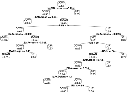
Fine! We have our first decision tree, let's see what we built.
If you want to play on your own with visualization, here’s a great resource.
A small note on the interpretation of this tree: nodes represent splitting, where the left branch reflects the answer “yes”, and the right branch answers “no”. The number in the final sheet is the percentage of cases that were correctly classified by this node.
Decision trees can also be used to select and evaluate indicators. The indicators, which are closer to the root (top) of the tree, give more divisions and contain more information than those at the bottom of the tree. In our case, the Stochastic Oscillator did not even hit the tree!
Although we have a set of rules that you can follow, you should still make sure that we have not retrained the model, so let's prune the tree. The easiest way to do this is to look at the complexity parameter, which is “cost,” or degraded performance. To do this, we need to add another division and choose the size of the tree, which minimizes our cross-validation error.
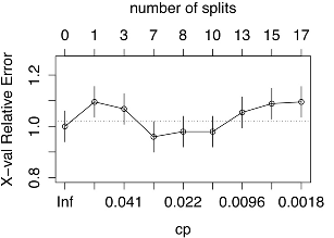
You can see that the smallest error is achieved for a tree of 7 partitions. Thanks to the cross-validation mode, which randomly selects data to test the model, your result may differ from the one shown in the screenshot. One of the drawbacks of the decision tree is that they may not be stable, i.e. small changes in data can lead to big changes in the tree. Therefore, the process of "trimming" the tree and other ways to prevent retraining are so important.
Let's cut this tree and see what our strategy will look like.
Now the tree looks like this:

So much better! Here you can see that the MACD signal line is no longer used. We started with 4 indicators, of which only a 3-day RSI, the difference between prices, and a 5-day EMA can be helpful in predicting price movements.
It's time to test the model on test data.
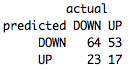
In general, not bad, 52% accuracy. More importantly, you have a basic strategy with well-defined, mathematical parameters. Using only 25 teams, we were able to determine which indicators are useful and what special conditions we need to complete the transaction. Now you can use these indicators for your own trading or to improve the tree.
In the next article, we will look at another powerful machine learning algorithm, the support vector machine, and figure out how to use its results for an even more robust strategy.
How to use decision tree for stock trading Bank of America.
Suppose you like to use a variety of technical indicators and you want to create a strategy that looks for specific high-probability opportunities in the market. What if the RSI value is above 85 and, at the same time, the MACD line below 20, means a good opportunity to open a short position? You can spend days / weeks / months in attempts to manually calculate all combinations of your indicators, or you can use a decision tree - a powerful and easily interpretable algorithm.
')
First, let's look at how decision trees work, then consider their use for the example of building a stock trading strategy of Bank of America.
How the decision tree works
Decision trees are one of the most popular machine learning algorithms, since they allow you to simulate data with strong noise, easily select non-linear trends, and catch the relationship between your indicators. However, they are also easily interpretable. Decision trees use a downstream, divide and conquer approach to data analysis. They look for an indicator and an indicator value that best breaks data into two opposite groups. The algorithm then repeats this process on each of the groups, and so it continues until it classifies each data point or the stopping criterion is reached. In our case, the data may belong to one of two groups: “Up” or “Down”. Each splitting, called a node, tries to maximize the purity of the resulting branches. Purity in this case is the probability that the data belong to one of the groups; it is characterized by the complexity parameter for each node.
Decision trees can easily retrain on test data and give a terrible result on new data. There are three ways to solve this problem:
• You can control the growth of the tree by specifying the threshold of the complexity parameter or the minimum number of data points in each branch, to fix the subset. This creates a tree that will try to cover wider models and will not focus on small subsets that may be unique to your data set.
• You can also prune trees after they have been built. This is usually done by choosing the size of the tree, which minimizes the cross-validation error. Cross-validation is a process that divides data into several groups, then uses all groups except one to build a model, and uses the remaining group of data to test the model. Then this process is repeated in such a way that each group is used for testing. Then the tree with the lowest average error is selected. This method is also good for preventing retraining if you have a limited amount of data.
• The most difficult way is to build many different trees and use them together to make decisions. There are three popular methods for building more than one decision tree: “bag”, “raised” trees, and random forests. Perhaps in future articles we will look at these methods in more detail.
Now that we have a basic understanding of decision trees, let's build our strategy!
Strategy building
Let's take a look at how to build a strategy based on 4 technical indicators to determine the movement of BoA stocks.
First, let's make sure that we have all the necessary libraries.
install.packages("quantmod") library("quantmod") # install.packages("rpart") library("rpart") # , . install.packages("rpart.plot") library("rpart.plot") # Then, let's get the data and calculate the indicators.
startDate = as.Date("2012-01-01") # endDate = as.Date("2014-01-01") # getSymbols("BAC", src = "yahoo", from = startDate, to = endDate) # Bank of America RSI3<-RSI(Op(BAC), n= 3) # 3- (RSI) EMA5<-EMA(Op(BAC),n=5) # 5- (EMA) EMAcross<- Op(BAC)-EMA5 # 5- EMA MACD<-MACD(Op(BAC),fast = 12, slow = 26, signal = 9) # MACD(/ ) MACDsignal<-MACD[,2] # SMI<-SMI(Op(BAC),n=13,slow=25,fast=2,signal=9) # SMI<-SMI[,1] # Then we calculate the variable that we predict and form the data sets.
PriceChange<- Cl(BAC) - Op(BAC) # Class<-ifelse(PriceChange>0,"UP","DOWN") # . DataSet<-data.frame(RSI3,EMAcross,MACDsignal,SMI,Class) # data set colnames(DataSet)<-c("RSI3","EMAcross","MACDsignal","Stochastic","Class") # DataSet<-DataSet[-c(1:33),] # , TrainingSet<-DataSet[1:312,] # 2/3 TestSet<-DataSet[313:469,] # 1/3 Now that we have everything we need, let's build this tree already!
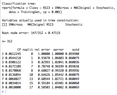
DecisionTree<-rpart(Class~RSI3+EMAcross+MACDsignal+Stochastic,data=TrainingSet, cp=.001) # , , (), . Fine! We have our first decision tree, let's see what we built.
prp(DecisionTree,type=2,extra=8) # , . 
If you want to play on your own with visualization, here’s a great resource.
A small note on the interpretation of this tree: nodes represent splitting, where the left branch reflects the answer “yes”, and the right branch answers “no”. The number in the final sheet is the percentage of cases that were correctly classified by this node.
Decision trees can also be used to select and evaluate indicators. The indicators, which are closer to the root (top) of the tree, give more divisions and contain more information than those at the bottom of the tree. In our case, the Stochastic Oscillator did not even hit the tree!
Although we have a set of rules that you can follow, you should still make sure that we have not retrained the model, so let's prune the tree. The easiest way to do this is to look at the complexity parameter, which is “cost,” or degraded performance. To do this, we need to add another division and choose the size of the tree, which minimizes our cross-validation error.
printcp(DecisionTree) # cp( ) , plotcp(DecisionTree,upper="splits") # 

You can see that the smallest error is achieved for a tree of 7 partitions. Thanks to the cross-validation mode, which randomly selects data to test the model, your result may differ from the one shown in the screenshot. One of the drawbacks of the decision tree is that they may not be stable, i.e. small changes in data can lead to big changes in the tree. Therefore, the process of "trimming" the tree and other ways to prevent retraining are so important.
Let's cut this tree and see what our strategy will look like.
PrunedDecisionTree<-prune(DecisionTree,cp=0.0272109) # (cp), (xerror) Now the tree looks like this:
prp(PrunedDecisionTree, type=2, extra=8) 
So much better! Here you can see that the MACD signal line is no longer used. We started with 4 indicators, of which only a 3-day RSI, the difference between prices, and a 5-day EMA can be helpful in predicting price movements.
It's time to test the model on test data.
table(predict(PrunedDecisionTree,TestSet,type="class"),TestSet[,5],dnn=list('predicted','actual')) 
In general, not bad, 52% accuracy. More importantly, you have a basic strategy with well-defined, mathematical parameters. Using only 25 teams, we were able to determine which indicators are useful and what special conditions we need to complete the transaction. Now you can use these indicators for your own trading or to improve the tree.
In the next article, we will look at another powerful machine learning algorithm, the support vector machine, and figure out how to use its results for an even more robust strategy.
Source: https://habr.com/ru/post/236769/
All Articles