Automatic optimization of algorithms using fast exponentiation of matrices
Suppose we want to calculate the ten millionth Fibonacci number in a Python program. A function that uses the trivial algorithm on my computer will perform calculations for more than 25 minutes. But if you apply a special optimizing decorator to the function, the function will calculate the answer in just 18 seconds ( 85 times faster ):

The fact is that before executing the program, the Python interpreter compiles all its parts into a special bytecode. Using the method described by habrip SkidanovAlex, this decorator analyzes the resulting byte-code of the function and tries to optimize the algorithm used there. Further you will see that this optimization can accelerate the program not as many times as it needs, but asymptotically. So, the greater the number of iterations in a cycle, the more times the optimized function will accelerate compared to the original.
This article will tell you about when and how the decorator manages to do such optimizations. You can also download and test the cpmoptimize library containing this decorator.
Two years ago, SkidanovAlex published an interesting article describing a limited language interpreter that supports the following operations:
The values of variables in the language must be numbers, their size is not limited ( long arithmetic is supported). In fact, variables are stored as integers in Python, which switches to long arithmetic mode if the number goes beyond the bounds of a hardware supported four or eight-byte type.
')
Consider the case when long arithmetic is not used. Then the execution time of the operations will not depend on the values of the variables, which means that in a cycle all iterations will be executed in the same time. If to execute such code "in the forehead", as in usual interpreters, the cycle will be executed in time. where n is the number of iterations. In other words, if the code for n iterations runs in time t , then the code for
  iterations will work for time
  (see computational complexity ).
The interpreter from the original article represents each variable operation supported by the language in the form of a definite matrix by which the vector with the initial values of the variables is multiplied. As a result of multiplication, we get a vector with new values of variables:
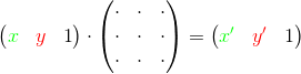
Thus, to perform a sequence of operations, one must multiply the vector in turn by the matrix corresponding to the next operation. Another way is by using associativity, the matrices can be multiplied first, and then the original vector can be multiplied by the resulting product:

To perform a cycle, we must calculate the number n , the number of iterations in the cycle, and also the matrix B , the sequential product of matrices corresponding to the operations from the cycle body. Then you need to multiply the source vector by the matrix B n times. Another way is to first raise the matrix B to the power n , and then multiply the vector with variables by the result:

If we use the binary exponentiation algorithm at that, the cycle can be performed in much less time. . So, if the code for n iterations works in time t , then the code for iterations will work for time
  (only two times slower, not n times slower, as in the previous case).
As a result, as was written above, the greater the number of iterations in the cycle n , the more times the optimized function is accelerated. Therefore, the effect of optimization will be especially noticeable for large n .
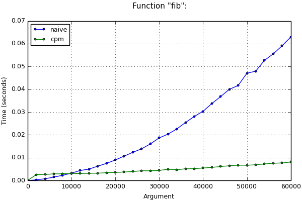
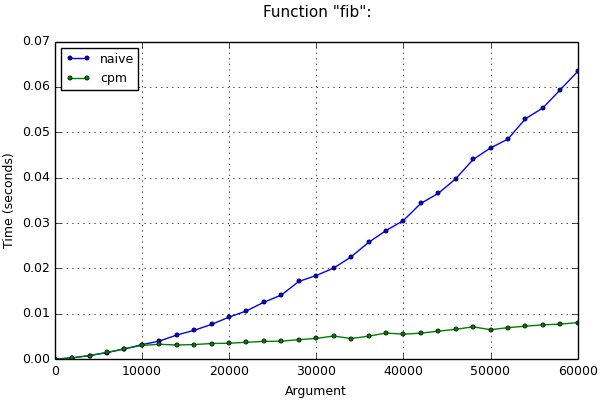
If long arithmetic is still used, the time estimates above may be incorrect. For example, when calculating the nth Fibonacci number, the values of variables from iteration to iteration become more and more, and operations with them are slowed down. The asymptotic estimate of the program operation time in such a case is more difficult to do (it is necessary to take into account the length of numbers in variables at each iteration and the methods used to multiply the numbers) and here it will not be given. However, after applying this optimization method, the asymptotics improves even in this case. This is clearly seen on the chart:
If tens of years ago a programmer would need to multiply a variable in a program by 4, he would not use the multiplication operation, but its faster equivalent - a bit left shift by 2. Now the compilers can do such optimizations themselves. In the struggle to reduce development time, languages with a high level of abstraction, new convenient technologies and libraries have appeared. When writing programs, more and more of their time is spent by developers on explaining to the computer what a program should do (multiply the number by 4), and not how to do it effectively (use a bit shift). Thus, the task of creating efficient code is partially transferred to compilers and interpreters.
Now compilers are able to replace various operations with more efficient ones, predict the values of expressions, delete or swap parts of the code. But compilers do not yet replace the computational algorithm written by man with the asymptotically more efficient one.
The implementation of the described method, presented in the original article, is problematic to use in real programs, since for this you will have to rewrite part of the code into a special language, and to interact with this code you will have to run a third-party script with an interpreter. However, the author of the article suggests using his work in practice in optimizing compilers. I tried to implement this method to optimize Python programs in a form that is really suitable for use in real projects.
If you use the library written by me, to apply the optimization, it will be enough to add one line before the function that needs to be accelerated using a special decorator. This decorator independently optimizes the cycles, if possible, and under no circumstances “breaks” the program.
Consider a series of tasks in which our decorator can be useful.
Suppose we have a certain sequence corresponding to the rule shown in the diagram, and we need to calculate its nth term:
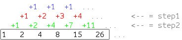
In this case, it is intuitively clear how the next member of the sequence appears, however, it takes time to come up with and prove the corresponding mathematical formula. Nevertheless, we can write a trivial algorithm describing our rule and suggest the computer to figure out how to quickly calculate the answer to our problem:
Interestingly, if you run this function for , inside it will run a loop with
  iterations. Without optimization, such a function would not work for any conceivable period of time, but with the decorator it is performed for less than a second, while returning the correct result.
To quickly calculate the nth Fibonacci number, there is a fast, but non-trivial algorithm based on the same idea of raising matrices to a power. An experienced developer can implement it in a few minutes. If the code where such calculations are made does not need to work quickly (for example, if you need to calculate the Fibonacci number with a number less than 10 thousand once), to save your working time, the developer will most likely decide to save efforts and write the solution “in forehead".
If the program still has to work quickly, or you have to make an effort and write a complex algorithm, or you can use the automatic optimization method, applying our decorator to the function. If n is large enough, in both cases the program performance will be almost the same, but in the second case the developer will spend less than his working time.
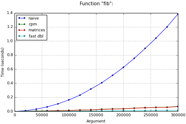
You can compare the working times of the described methods below on tables and graphs for small and for large n .
To be fair, it should be noted that to calculate the Fibonacci numbers there is another algorithm known as fast doubling . He somewhat wins the previous algorithms in time, since it eliminates unnecessary additions and multiplications of numbers. The computation time through this algorithm is also presented in the graphs for comparison.
In practice, we can meet with a more complex situation if the sequence of numbers instead of the well-known recurrent formula:
It is given by a somewhat complicated formula, for example, this:

In this case, we will not be able to find the implementation of the above algorithms on the Internet, and it will take significant time to manually come up with an algorithm to raise matrices to a power. Nevertheless, we can write a solution "in the forehead" and apply a decorator, then the computer will come up with a fast algorithm for us:
Suppose we need to calculate the sum of the count members of the geometric progression, for which the first member start and the denominator of coeff are given . In this task, the decorator is again able to optimize our trivial solution:
Suppose we need to raise the number a to a nonnegative integer power n . In such a task, the decorator will actually replace the trivial solution with the binary exponentiation algorithm:
You can install the library using pip :
The source code for the library with examples is available on github under a free MIT license.
UPD. The package is published in the Python Package Index.
Examples of the use of optimization are in the " tests / " folder. Each example consists of a function representing the solution "in the forehead", its optimized version, as well as functions representing the well-known complex, but quick solutions of this problem. These functions are placed in scripts that run them on different groups of tests, measure the time of their work and build the corresponding tables. If the matplotlib library is installed , the scripts will also build graphs of the dependence of the running time of the functions on the input data (regular or logarithmic) and save them in the " tests / plots / " folder.
When creating the library, I used the fact that the byte-code of the program that the Python interpreter creates can be analyzed and modified at the execution stage without interfering with the interpreter, which gives wide possibilities for language extension (see, for example, the goto implementation ). The advantages of the described method usually manifest themselves when using long arithmetic, which is also built into Python.
For these reasons, the implementation of the described optimization in Python has become a more interesting task for me, although, of course, its use in C ++ compilers would allow creating even faster programs. In addition, the decoder-optimized Python code, as a rule, overtakes the head-on code in C ++ due to better asymptotics.
When modifying the bytecode, I used the byteplay module, which provides a convenient interface for disassembling and assembling bytecode. Unfortunately, the module has not yet been ported to Python 3, so I implemented the entire project in Python 2.7.
The name of the cpmoptimize library is an abbreviation of the words " c ompute and optimize " . The size of the article does not allow to describe in detail the process of analysis and modification of the byte-code, however, I will try to describe in detail what features this library provides and on what principles its work is based.
cpmoptimize. xrange ( stop )
cpmoptimize. xrange ( start , stop [, step ])
The built-in type xrange in Python 2 for optimization does not support long integers of type long as arguments:
Since when using our library cycles with the number of operations of the order can be executed in less than a second, and become a routine in the program, the library provides its own xrange implementation in pure Python (inside the library it is called CPMRange ). It supports all the capabilities of the usual xrange and, in addition, the arguments of the type long . Such code will not lead to errors and quickly calculate the correct result:
However, if in your case the number of iterations in the cycles is small, you can continue to use the built-in xrange with the decorator.
cpmoptimize. cpmoptimize ( strict = False, iters_limit = 5000, types = (int, long), opt_min_rows = True, opt_clear_stack = True)
The cpmoptimize function takes the parameters of the optimization performed and returns a decorator that takes these parameters into account, which we need to apply to the function being optimized. This can be done using a special syntax (with the “dog” symbol) or without it:
Before making changes to the bytecode, the original function is copied. Thus, in the above code, the functions f and smart_g will eventually be optimized, but naive_g will not.
The decorator searches the byte-code of the function for standard loops, while loops while for loops and for loops inside the generator and list expressions are ignored. Nested loops are not yet supported (only the innermost loop is optimized). Properly processed for-else constructions .
The decorator cannot optimize the cycle, regardless of what types of variables are used in it. The fact is that, for example, Python allows you to define a type that, with each multiplication, writes a string to a file. As a result of applying the optimization, the number of multiplications made in the function could change. Because of this, the number of lines in the file would be different and optimization would break the program.
In addition, during matrix operations, variables are added and multiplied implicitly, so the types of variables can be “mixed”. If one of the constants or variables would be of type float , those variables that would have to be of type int after executing the code could also get a type of float (since the addition of int and float returns a float ). This behavior can cause errors in the program and is also unacceptable.
To avoid unwanted side effects, the decorator optimizes the cycle only if all the constants and variables used in it have a valid type. Initially, the valid types are int and long , as well as the types inherited from them. If one of the constants or variables is of the long type, those variables that would have had the int type after the execution of the code can also get the long type. However, since int and long in Python are fairly interchangeable, this should not lead to errors.
In case you want to change the set of valid types (for example, to add float support), you must pass a tuple of the required types in the types parameter. Types included in this tuple or inherited from the types included in this tuple will be considered valid. In fact, checking that a value has a valid type will be done using the expression isinstance (value, types) .
Each cycle found should satisfy a number of conditions. Some of them are checked already when applying the decorator:
If these conditions are met, a “trap” is set before the cycle, which checks another part of the conditions, and the original byte-code of the cycle is not deleted. Since Python uses dynamic typing, the following conditions can be checked only immediately before the loop starts:
If the “trap” concluded that the optimization is acceptable, the necessary matrices will be calculated, and then the values of the variables used will change to new ones. If optimization cannot be performed, the original bytecode of the loop will be launched.
Although the described method does not support exponentiation and “bitwise AND” operations, the following code will be optimized:
When analyzing the byte-code, the decorator will conclude that the values of the variables k and m in the expression (k ** m) & 676 do not depend on which iteration of the cycle they are used, and therefore the value of the whole expression does not change. It is not necessary to calculate it at each iteration; it is enough to calculate this value once. Therefore, the corresponding instructions of the byte-code can be taken out and executed them immediately before the start of the cycle, substituting the ready-made value in the cycle. The code will be as if converted to the following:
This technique is known as the removal of the invariant code loop ( loop-invariant code motion ).Note that the offset values are calculated each time the function is started, since they can depend on changing global variables or function parameters (like _const1 in the example depends on the parameter k ). The resulting code is now easy to optimize using matrices.
It is at this stage that the predictability of the values described above is performed. For example, if one of the “bitwise AND” operands were unpredictable, this operation could no longer be taken out of the loop and optimization could not be applied.
The decorator also partially supports multiple assignments. If there are few elements in them, Python creates a byte code supported by the decorator without using tuples:
In the graphs above, you may have noticed that with a small number of iterations, the optimized cycle may work slower than usual, since in this case it still takes some time to construct the matrices and check the types. In cases where it is necessary for the function to work as quickly as possible and with a small number of iterations, you can explicitly set the threshold by the iters_limit parameter . Then the “trap” before starting the optimization will check how many iterations the loop will have to perform, and will cancel the optimization if this number does not exceed the specified threshold.
Initially, the threshold is set at 5000 iterations. It cannot be set lower than in 2 iterations.
It is clear that the most favorable threshold value is the intersection point on the graph of lines corresponding to the operating time of the optimized and initial variants of the function. If you set the threshold exactly this way, the function will be able to choose the fastest in this case algorithm (optimized or initial):
In some cases, optimization should be mandatory applied. So, if in a cycle ofiterations, without optimization, the program will simply hang. The strict option is provided for this case . Initially, its value is False , but if it is set to True , then in the case when any of the standard for loops has not been optimized, an exception will be raised.
If the fact that optimization is not applicable, was discovered at the stage of applying the decorator, the exception cpmoptimize.recompiler.RecompilationError will be raised immediately . In the example in the cycle, two unpredictable variables are multiplied:
If the fact that optimization is not applicable was detected before executing the loop (that is, if it turned out that the types of values of the iterator or variables are not supported), a TypeError exception will be raised :
Two flags opt_min_rows and opt_clear_stack are responsible for using additional optimization methods when constructing matrices. Initially they are included, the possibility of their disconnection is present only for demonstration purposes (thanks to it, it is possible to compare the effectiveness of these methods).
When executing an optimized code, most of the time is the multiplication of long numbers in some cells of the generated matrices. Compared with this time-consuming process, the time spent on multiplying all the other cells is negligible.
In the process of recompiling expressions, the decorator creates intermediate, virtualvariables responsible for the positions of the interpreter stack. After complex calculations, they can have long numbers that are already stored in some other, real variables. We don’t need to store these values a second time, but they remain in the cells of the matrix and significantly slow down the work of the program, since when multiplying matrices we have to multiply these long numbers once more. The opt_clear_stack option is responsible for clearing such variables: if after they are used, they are set to zero, the long values in them will disappear.
This option is especially effective when the program operates with very large numbers. The elimination of unnecessary multiplications of such numbers makes it possible to speed up the program more than twice. Opt_min_rows
optionincludes minimizing the size of square matrices that we multiply. Rows corresponding to unused and predictable variables are excluded from the matrices. If the loop variable itself is not used, the rows responsible for maintaining its correct value are also excluded. In order not to disrupt the program, after the cycle, all these variables will be assigned the correct final values. In addition, in the original article, the vector of variables was supplemented with an element equal to one. If the row corresponding to this element is unused, it will also be excluded.
This option can speed up the program somewhat for not very large n , when the numbers have not yet become very long and the dimensions of the matrix make a tangible contribution during the operation of the program.
If both options are used simultaneously, the virtual variables start to have a predictable (zero) value, and opt_min_rows works even more efficiently. In other words, the effectiveness of both options together is greater than the effectiveness of each of them separately.
The graph below shows the program runtime for calculating Fibonacci numbers when certain options are disabled (here "-m" is a program with opt_min_rows turned off , "-c" is a program with opt_clear_stack disabled , "-mc" is a program where both options are disabled ):

We will say that our method supports a couple of operations if:
if:
We already know that the method supports a couple of operations. . Really:
These operations are currently implemented in the optimizing decorator. However, it turns out that the described method supports other pairs of operations, including (a pair of multiplication and exponentiation operations).
For example, our task may be to find the nth number in the sequence given by the recurrence relation:
If our decorator supported a couple of operations, we could multiply the variable by another variable (but could not add the variables anymore). In this case, the following trivial solution of this problem could be speeded up by the decorator:
It can be proved that our method also supports pairs of operations. ,
,  and
and  (here and is bitwise AND, or - bitwise OR). In the case of positive numbers you can work with pairs of operations
 and
and  .
.
To implement support for operations,you can, for example, operate not with the values of variables, but with logarithms of these values. Then the multiplication of variables is replaced by the addition of logarithms, and the raising of a variable to a constant degree by the multiplication of the logarithm by a constant. Thus, we will reduce the task to the already realized case with operations. .
The explanation of how to implement support for the remaining pairs of operations mentioned above contains a number of mathematical calculations and is worthy of a separate article. At the moment it is only worth mentioning that pairs of operations are interchangeable to a certain extent.
Having improved the algorithm for analyzing loops in bytecode, you can implement support for nested loops in order to optimize code like this:
In the following code, the condition in the body of the loop is predictable. You can even find out if it is true before starting the loop and remove the non-executing code branch. The resulting code can be optimized:
The Python interpreter, generally speaking, creates a predictable bytecode that almost exactly matches the source code you wrote. Standardly, it does not embed functions, nor does it unfold loops, nor any other optimizations that require an analysis of the behavior of the program. Only since version 2.6, CPython has learned to minimize constant arithmetic expressions, but this feature does not always work effectively.
There are several reasons for this situation. First, code analysis is generally difficult in Python, because you can track data types only during program execution (which we do in our case). Secondly, optimization, as a rule, still does not allow Python to reach the speed of purely compiled languages, so in the case when the program needs to work very quickly, it is suggested to simply write it in a lower level language.
Nevertheless, Python is a flexible language, which allows, if necessary, to implement many optimization methods independently without interfering with the interpreter. This library, as well as other projects listed below, illustrate this opportunity well.
UPD.The project description is now also available as a SlideShare presentation .
Below I will provide links to several other interesting projects to speed up the execution of Python programs:
UPD # 1. The user magik offered some more links:
UPD # 2. User DuneRat pointed to several more Python compilation projects: shedskin , hope , pythran .
The fact is that before executing the program, the Python interpreter compiles all its parts into a special bytecode. Using the method described by habrip SkidanovAlex, this decorator analyzes the resulting byte-code of the function and tries to optimize the algorithm used there. Further you will see that this optimization can accelerate the program not as many times as it needs, but asymptotically. So, the greater the number of iterations in a cycle, the more times the optimized function will accelerate compared to the original.
This article will tell you about when and how the decorator manages to do such optimizations. You can also download and test the cpmoptimize library containing this decorator.
Theory
Two years ago, SkidanovAlex published an interesting article describing a limited language interpreter that supports the following operations:
# x = y x = 1 # x += y x += 2 x -= y x -= 3 # x *= 4 # loop 100000 ... end The values of variables in the language must be numbers, their size is not limited ( long arithmetic is supported). In fact, variables are stored as integers in Python, which switches to long arithmetic mode if the number goes beyond the bounds of a hardware supported four or eight-byte type.
')
Consider the case when long arithmetic is not used. Then the execution time of the operations will not depend on the values of the variables, which means that in a cycle all iterations will be executed in the same time. If to execute such code "in the forehead", as in usual interpreters, the cycle will be executed in time.
where n is the number of iterations. In other words, if the code for n iterations runs in time t , then the code for iterations will work for time (see computational complexity ).The interpreter from the original article represents each variable operation supported by the language in the form of a definite matrix by which the vector with the initial values of the variables is multiplied. As a result of multiplication, we get a vector with new values of variables:
Thus, to perform a sequence of operations, one must multiply the vector in turn by the matrix corresponding to the next operation. Another way is by using associativity, the matrices can be multiplied first, and then the original vector can be multiplied by the resulting product:
To perform a cycle, we must calculate the number n , the number of iterations in the cycle, and also the matrix B , the sequential product of matrices corresponding to the operations from the cycle body. Then you need to multiply the source vector by the matrix B n times. Another way is to first raise the matrix B to the power n , and then multiply the vector with variables by the result:
If we use the binary exponentiation algorithm at that, the cycle can be performed in much less time.
. So, if the code for n iterations works in time t , then the code for iterations will work for time (only two times slower, not n times slower, as in the previous case).As a result, as was written above, the greater the number of iterations in the cycle n , the more times the optimized function is accelerated. Therefore, the effect of optimization will be especially noticeable for large n .
If long arithmetic is still used, the time estimates above may be incorrect. For example, when calculating the nth Fibonacci number, the values of variables from iteration to iteration become more and more, and operations with them are slowed down. The asymptotic estimate of the program operation time in such a case is more difficult to do (it is necessary to take into account the length of numbers in variables at each iteration and the methods used to multiply the numbers) and here it will not be given. However, after applying this optimization method, the asymptotics improves even in this case. This is clearly seen on the chart:
Idea
If tens of years ago a programmer would need to multiply a variable in a program by 4, he would not use the multiplication operation, but its faster equivalent - a bit left shift by 2. Now the compilers can do such optimizations themselves. In the struggle to reduce development time, languages with a high level of abstraction, new convenient technologies and libraries have appeared. When writing programs, more and more of their time is spent by developers on explaining to the computer what a program should do (multiply the number by 4), and not how to do it effectively (use a bit shift). Thus, the task of creating efficient code is partially transferred to compilers and interpreters.
Now compilers are able to replace various operations with more efficient ones, predict the values of expressions, delete or swap parts of the code. But compilers do not yet replace the computational algorithm written by man with the asymptotically more efficient one.
The implementation of the described method, presented in the original article, is problematic to use in real programs, since for this you will have to rewrite part of the code into a special language, and to interact with this code you will have to run a third-party script with an interpreter. However, the author of the article suggests using his work in practice in optimizing compilers. I tried to implement this method to optimize Python programs in a form that is really suitable for use in real projects.
If you use the library written by me, to apply the optimization, it will be enough to add one line before the function that needs to be accelerated using a special decorator. This decorator independently optimizes the cycles, if possible, and under no circumstances “breaks” the program.
Examples of using
Consider a series of tasks in which our decorator can be useful.
Example number 1. Long cycles
Suppose we have a certain sequence corresponding to the rule shown in the diagram, and we need to calculate its nth term:
In this case, it is intuitively clear how the next member of the sequence appears, however, it takes time to come up with and prove the corresponding mathematical formula. Nevertheless, we can write a trivial algorithm describing our rule and suggest the computer to figure out how to quickly calculate the answer to our problem:
from cpmoptimize import cpmoptimize, xrange @cpmoptimize() def f(n): step1 = 1 step2 = 1 res = 1 for i in xrange(n): res += step2 step2 += step1 step1 += 1 return res Interestingly, if you run this function for
, inside it will run a loop with iterations. Without optimization, such a function would not work for any conceivable period of time, but with the decorator it is performed for less than a second, while returning the correct result.Example number 2. Fibonacci numbers
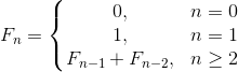
To quickly calculate the nth Fibonacci number, there is a fast, but non-trivial algorithm based on the same idea of raising matrices to a power. An experienced developer can implement it in a few minutes. If the code where such calculations are made does not need to work quickly (for example, if you need to calculate the Fibonacci number with a number less than 10 thousand once), to save your working time, the developer will most likely decide to save efforts and write the solution “in forehead".
If the program still has to work quickly, or you have to make an effort and write a complex algorithm, or you can use the automatic optimization method, applying our decorator to the function. If n is large enough, in both cases the program performance will be almost the same, but in the second case the developer will spend less than his working time.
You can compare the working times of the described methods below on tables and graphs for small and for large n .
To be fair, it should be noted that to calculate the Fibonacci numbers there is another algorithm known as fast doubling . He somewhat wins the previous algorithms in time, since it eliminates unnecessary additions and multiplications of numbers. The computation time through this algorithm is also presented in the graphs for comparison.
Charts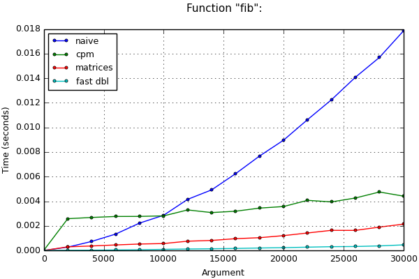
Time measurement results
Function "fib": (*) Testcase "big": +--------+----------+--------------+--------------+--------------+-------+ | arg | naive, s | cpm, s | matrices, s | fast dbl, s | match | +--------+----------+--------------+--------------+--------------+-------+ | 0 | 0.00 | 0.00 | 0.00 | 0.00 | True | | 20000 | 0.01 | 0.00 (2.5x) | 0.00 (3.0x) | 0.00 (5.1x) | True | | 40000 | 0.03 | 0.01 (5.7x) | 0.00 (1.8x) | 0.00 (4.8x) | True | | 60000 | 0.06 | 0.01 (7.9x) | 0.01 (1.4x) | 0.00 (4.8x) | True | | 80000 | 0.11 | 0.01 (9.4x) | 0.01 (1.3x) | 0.00 (4.6x) | True | | 100000 | 0.16 | 0.01 (11.6x) | 0.01 (1.1x) | 0.00 (4.5x) | True | | 120000 | 0.23 | 0.02 (11.8x) | 0.02 (1.2x) | 0.00 (4.7x) | True | | 140000 | 0.32 | 0.02 (14.7x) | 0.02 (1.1x) | 0.00 (4.1x) | True | | 160000 | 0.40 | 0.03 (13.1x) | 0.03 (1.2x) | 0.01 (4.6x) | True | | 180000 | 0.51 | 0.03 (14.7x) | 0.03 (1.1x) | 0.01 (4.4x) | True | | 200000 | 0.62 | 0.04 (16.6x) | 0.03 (1.1x) | 0.01 (4.4x) | True | | 220000 | 0.75 | 0.05 (16.1x) | 0.04 (1.1x) | 0.01 (4.9x) | True | | 240000 | 0.89 | 0.05 (17.1x) | 0.05 (1.0x) | 0.01 (4.7x) | True | | 260000 | 1.04 | 0.06 (18.1x) | 0.06 (1.0x) | 0.01 (4.5x) | True | | 280000 | 1.20 | 0.06 (20.2x) | 0.06 (1.0x) | 0.01 (4.2x) | True | | 300000 | 1.38 | 0.07 (19.4x) | 0.07 (1.1x) | 0.02 (4.4x) | True | +--------+----------+--------------+--------------+--------------+-------+ In practice, we can meet with a more complex situation if the sequence of numbers instead of the well-known recurrent formula:
It is given by a somewhat complicated formula, for example, this:
In this case, we will not be able to find the implementation of the above algorithms on the Internet, and it will take significant time to manually come up with an algorithm to raise matrices to a power. Nevertheless, we can write a solution "in the forehead" and apply a decorator, then the computer will come up with a fast algorithm for us:
from cpmoptimize import cpmoptimize @cpmoptimize() def f(n): prev3 = 0 prev2 = 1 prev1 = 1 for i in xrange(3, n + 3): cur = 7 * (2 * prev1 + 3 * prev2) + 4 * prev3 + 5 * i + 6 prev3, prev2, prev1 = prev2, prev1, cur return prev3 Example number 3. Sum of a geometric progression
Suppose we need to calculate the sum of the count members of the geometric progression, for which the first member start and the denominator of coeff are given . In this task, the decorator is again able to optimize our trivial solution:
from cpmoptimize import cpmoptimize @cpmoptimize() def geom_sum(start, coeff, count): res = 0 elem = start for i in xrange(count): res += elem elem *= coeff return res Schedule
Example number 4. Exponentiation
Suppose we need to raise the number a to a nonnegative integer power n . In such a task, the decorator will actually replace the trivial solution with the binary exponentiation algorithm:
from cpmoptimize import cpmoptimize @cpmoptimize() def power(a, n): res = 1 for i in xrange(n): res *= a return res Schedule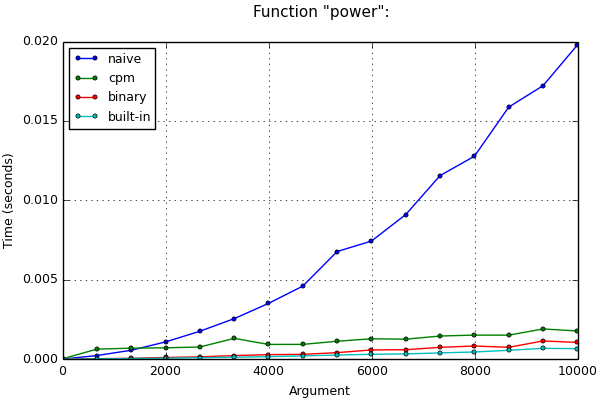
Download links
You can install the library using pip :
sudo pip install cpmoptimize The source code for the library with examples is available on github under a free MIT license.
UPD. The package is published in the Python Package Index.
Examples of the use of optimization are in the " tests / " folder. Each example consists of a function representing the solution "in the forehead", its optimized version, as well as functions representing the well-known complex, but quick solutions of this problem. These functions are placed in scripts that run them on different groups of tests, measure the time of their work and build the corresponding tables. If the matplotlib library is installed , the scripts will also build graphs of the dependence of the running time of the functions on the input data (regular or logarithmic) and save them in the " tests / plots / " folder.
Library Description
When creating the library, I used the fact that the byte-code of the program that the Python interpreter creates can be analyzed and modified at the execution stage without interfering with the interpreter, which gives wide possibilities for language extension (see, for example, the goto implementation ). The advantages of the described method usually manifest themselves when using long arithmetic, which is also built into Python.
For these reasons, the implementation of the described optimization in Python has become a more interesting task for me, although, of course, its use in C ++ compilers would allow creating even faster programs. In addition, the decoder-optimized Python code, as a rule, overtakes the head-on code in C ++ due to better asymptotics.
When modifying the bytecode, I used the byteplay module, which provides a convenient interface for disassembling and assembling bytecode. Unfortunately, the module has not yet been ported to Python 3, so I implemented the entire project in Python 2.7.
The name of the cpmoptimize library is an abbreviation of the words " c ompute and optimize " . The size of the article does not allow to describe in detail the process of analysis and modification of the byte-code, however, I will try to describe in detail what features this library provides and on what principles its work is based.
Own xrange
cpmoptimize. xrange ( stop )
cpmoptimize. xrange ( start , stop [, step ])
The built-in type xrange in Python 2 for optimization does not support long integers of type long as arguments:
>>> xrange(10 ** 1000) Traceback (most recent call last): File "<stdin>", line 1, in <module> OverflowError: Python int too large to convert to C long Since when using our library cycles with the number of operations of the order
can be executed in less than a second, and become a routine in the program, the library provides its own xrange implementation in pure Python (inside the library it is called CPMRange ). It supports all the capabilities of the usual xrange and, in addition, the arguments of the type long . Such code will not lead to errors and quickly calculate the correct result: from cpmoptimize import cpmoptimize, xrange @cpmoptimize() def f(): res = 0 for i in xrange(10 ** 1000): res += 3 return res print f() However, if in your case the number of iterations in the cycles is small, you can continue to use the built-in xrange with the decorator.
Cpmoptimize function
cpmoptimize. cpmoptimize ( strict = False, iters_limit = 5000, types = (int, long), opt_min_rows = True, opt_clear_stack = True)
Decorator application
The cpmoptimize function takes the parameters of the optimization performed and returns a decorator that takes these parameters into account, which we need to apply to the function being optimized. This can be done using a special syntax (with the “dog” symbol) or without it:
from cpmoptimize import cpmoptimize @cpmoptimize() def f(n): # def naive_g(n): # smart_g = cpmoptimize()(naive_g) Before making changes to the bytecode, the original function is copied. Thus, in the above code, the functions f and smart_g will eventually be optimized, but naive_g will not.
Search for loops
The decorator searches the byte-code of the function for standard loops, while loops while for loops and for loops inside the generator and list expressions are ignored. Nested loops are not yet supported (only the innermost loop is optimized). Properly processed for-else constructions .
Valid Types
The decorator cannot optimize the cycle, regardless of what types of variables are used in it. The fact is that, for example, Python allows you to define a type that, with each multiplication, writes a string to a file. As a result of applying the optimization, the number of multiplications made in the function could change. Because of this, the number of lines in the file would be different and optimization would break the program.
In addition, during matrix operations, variables are added and multiplied implicitly, so the types of variables can be “mixed”. If one of the constants or variables would be of type float , those variables that would have to be of type int after executing the code could also get a type of float (since the addition of int and float returns a float ). This behavior can cause errors in the program and is also unacceptable.
To avoid unwanted side effects, the decorator optimizes the cycle only if all the constants and variables used in it have a valid type. Initially, the valid types are int and long , as well as the types inherited from them. If one of the constants or variables is of the long type, those variables that would have had the int type after the execution of the code can also get the long type. However, since int and long in Python are fairly interchangeable, this should not lead to errors.
In case you want to change the set of valid types (for example, to add float support), you must pass a tuple of the required types in the types parameter. Types included in this tuple or inherited from the types included in this tuple will be considered valid. In fact, checking that a value has a valid type will be done using the expression isinstance (value, types) .
Cycle optimization conditions
Each cycle found should satisfy a number of conditions. Some of them are checked already when applying the decorator:
- The body of the loop should consist only of assignment instructions, unary and binary operations, which can be put together into complex expressions. It cannot contain conditions, calls to other functions, return or yield statements , etc.
- Predictability condition may be required from the operands: at each iteration of the loop, their value should be the same, and it should not depend on the results of any calculations at the previous iteration. Wherein:
- All operands of addition and subtraction, as well as the operand of a unary minus can be unpredictable.
- At least one multiplication operand must be predictable (similar to the fact that in the original interpreter only multiplication by a constant was supported).
- All operands of exponentiation, division, and taking of the remainder and bitwise operations must be predictable.
- All constants used in the loop must have a valid type.
If these conditions are met, a “trap” is set before the cycle, which checks another part of the conditions, and the original byte-code of the cycle is not deleted. Since Python uses dynamic typing, the following conditions can be checked only immediately before the loop starts:
- The object through which the loop is run must be of the standard type xrange or its equivalent from the given library cpmoptimize.xrange . However, the slow range function that returns a list is not supported.
- The values of all variables used in the loop are of a valid type.
If the “trap” concluded that the optimization is acceptable, the necessary matrices will be calculated, and then the values of the variables used will change to new ones. If optimization cannot be performed, the original bytecode of the loop will be launched.
Expressions and removal of code per cycle
Although the described method does not support exponentiation and “bitwise AND” operations, the following code will be optimized:
@cpmoptimize() def f(n, k): res = 0 for i in xrange(n): m = 3 res += ((k ** m) & 676) + i return res When analyzing the byte-code, the decorator will conclude that the values of the variables k and m in the expression (k ** m) & 676 do not depend on which iteration of the cycle they are used, and therefore the value of the whole expression does not change. It is not necessary to calculate it at each iteration; it is enough to calculate this value once. Therefore, the corresponding instructions of the byte-code can be taken out and executed them immediately before the start of the cycle, substituting the ready-made value in the cycle. The code will be as if converted to the following:
@cpmoptimize() def f(n, k): res = 0 m = 3 _const1 = (k ** m) & 676 for i in xrange(n): res += _const1 + i return res This technique is known as the removal of the invariant code loop ( loop-invariant code motion ).Note that the offset values are calculated each time the function is started, since they can depend on changing global variables or function parameters (like _const1 in the example depends on the parameter k ). The resulting code is now easy to optimize using matrices.
It is at this stage that the predictability of the values described above is performed. For example, if one of the “bitwise AND” operands were unpredictable, this operation could no longer be taken out of the loop and optimization could not be applied.
The decorator also partially supports multiple assignments. If there are few elements in them, Python creates a byte code supported by the decorator without using tuples:
a, b = b, a + b Threshold iters_limit
In the graphs above, you may have noticed that with a small number of iterations, the optimized cycle may work slower than usual, since in this case it still takes some time to construct the matrices and check the types. In cases where it is necessary for the function to work as quickly as possible and with a small number of iterations, you can explicitly set the threshold by the iters_limit parameter . Then the “trap” before starting the optimization will check how many iterations the loop will have to perform, and will cancel the optimization if this number does not exceed the specified threshold.
Initially, the threshold is set at 5000 iterations. It cannot be set lower than in 2 iterations.
It is clear that the most favorable threshold value is the intersection point on the graph of lines corresponding to the operating time of the optimized and initial variants of the function. If you set the threshold exactly this way, the function will be able to choose the fastest in this case algorithm (optimized or initial):
Strict flag
In some cases, optimization should be mandatory applied. So, if in a cycle of
iterations, without optimization, the program will simply hang. The strict option is provided for this case . Initially, its value is False , but if it is set to True , then in the case when any of the standard for loops has not been optimized, an exception will be raised.If the fact that optimization is not applicable, was discovered at the stage of applying the decorator, the exception cpmoptimize.recompiler.RecompilationError will be raised immediately . In the example in the cycle, two unpredictable variables are multiplied:
>>> from cpmoptimize import cpmoptimize >>> >>> @cpmoptimize(strict=True) ... def f(n, k): ... res = 0 ... for i in xrange(n): ... res += i * res ... return res ... Traceback (most recent call last): File "<stdin>", line 1, in <module> File "cpmoptimize/__init__.py", line 100, in upgrade_func index += analyze_loop(settings, code, index) + 1 File "cpmoptimize/__init__.py", line 59, in analyze_loop raise err cpmoptimize.recompiler.RecompileError: Multiplication of two unpredictable values is unsupported If the fact that optimization is not applicable was detected before executing the loop (that is, if it turned out that the types of values of the iterator or variables are not supported), a TypeError exception will be raised :
>>> from cpmoptimize import cpmoptimize >>> >>> @cpmoptimize(strict=True) ... def f(iterable): ... res = 0 ... for elem in iterable: ... res += elem ... return res ... >>> f(xrange(30)) 435 >>> f(range(30)) Traceback (most recent call last): File "<stdin>", line 1, in <module> File "<stdin>", line 4, in f File "cpmoptimize/hook.py", line 170, in exec_loop raise err TypeError: Iterator in optimized loops must have type "xrange" instead of <type 'list'> Advanced Optimization Options
Two flags opt_min_rows and opt_clear_stack are responsible for using additional optimization methods when constructing matrices. Initially they are included, the possibility of their disconnection is present only for demonstration purposes (thanks to it, it is possible to compare the effectiveness of these methods).
When executing an optimized code, most of the time is the multiplication of long numbers in some cells of the generated matrices. Compared with this time-consuming process, the time spent on multiplying all the other cells is negligible.
In the process of recompiling expressions, the decorator creates intermediate, virtualvariables responsible for the positions of the interpreter stack. After complex calculations, they can have long numbers that are already stored in some other, real variables. We don’t need to store these values a second time, but they remain in the cells of the matrix and significantly slow down the work of the program, since when multiplying matrices we have to multiply these long numbers once more. The opt_clear_stack option is responsible for clearing such variables: if after they are used, they are set to zero, the long values in them will disappear.
This option is especially effective when the program operates with very large numbers. The elimination of unnecessary multiplications of such numbers makes it possible to speed up the program more than twice. Opt_min_rows
optionincludes minimizing the size of square matrices that we multiply. Rows corresponding to unused and predictable variables are excluded from the matrices. If the loop variable itself is not used, the rows responsible for maintaining its correct value are also excluded. In order not to disrupt the program, after the cycle, all these variables will be assigned the correct final values. In addition, in the original article, the vector of variables was supplemented with an element equal to one. If the row corresponding to this element is unused, it will also be excluded.
This option can speed up the program somewhat for not very large n , when the numbers have not yet become very long and the dimensions of the matrix make a tangible contribution during the operation of the program.
If both options are used simultaneously, the virtual variables start to have a predictable (zero) value, and opt_min_rows works even more efficiently. In other words, the effectiveness of both options together is greater than the effectiveness of each of them separately.
The graph below shows the program runtime for calculating Fibonacci numbers when certain options are disabled (here "-m" is a program with opt_min_rows turned off , "-c" is a program with opt_clear_stack disabled , "-mc" is a program where both options are disabled ):
What else can be implemented?
Modifying a set of operations
We will say that our method supports a couple of operations
if:- We can perform an operation
 for two variables or for a variable and a constant;
 - We can perform an operation
 for a variable and a constant.
We already know that the method supports a couple of operations.
. Really:- We can add two variables or a variable and a constant;
- We can multiply a variable by a constant.
These operations are currently implemented in the optimizing decorator. However, it turns out that the described method supports other pairs of operations, including
(a pair of multiplication and exponentiation operations).For example, our task may be to find the nth number in the sequence given by the recurrence relation:
If our decorator supported a couple of operations
, we could multiply the variable by another variable (but could not add the variables anymore). In this case, the following trivial solution of this problem could be speeded up by the decorator: def f(n): a = 1 b = 1 for i in xrange(n): a, b = b, a * b return a It can be proved that our method also supports pairs of operations.
, and (here and is bitwise AND, or - bitwise OR). In the case of positive numbers you can work with pairs of operations and .To implement support for operations,
you can, for example, operate not with the values of variables, but with logarithms of these values. Then the multiplication of variables is replaced by the addition of logarithms, and the raising of a variable to a constant degree by the multiplication of the logarithm by a constant. Thus, we will reduce the task to the already realized case with operations. .The explanation of how to implement support for the remaining pairs of operations mentioned above contains a number of mathematical calculations and is worthy of a separate article. At the moment it is only worth mentioning that pairs of operations are interchangeable to a certain extent.
Nested loops
Having improved the algorithm for analyzing loops in bytecode, you can implement support for nested loops in order to optimize code like this:
def f(): res = 0 for i in xrange(10 ** 50): for j in xrange(10 ** 100): res += i * 2 + j return res Predictable conditions
In the following code, the condition in the body of the loop is predictable. You can even find out if it is true before starting the loop and remove the non-executing code branch. The resulting code can be optimized:
def f(mode): res = 0 for i in xrange(10 ** 50): if mode == 1: res += 3 else: res += 5 return res findings
The Python interpreter, generally speaking, creates a predictable bytecode that almost exactly matches the source code you wrote. Standardly, it does not embed functions, nor does it unfold loops, nor any other optimizations that require an analysis of the behavior of the program. Only since version 2.6, CPython has learned to minimize constant arithmetic expressions, but this feature does not always work effectively.
There are several reasons for this situation. First, code analysis is generally difficult in Python, because you can track data types only during program execution (which we do in our case). Secondly, optimization, as a rule, still does not allow Python to reach the speed of purely compiled languages, so in the case when the program needs to work very quickly, it is suggested to simply write it in a lower level language.
Nevertheless, Python is a flexible language, which allows, if necessary, to implement many optimization methods independently without interfering with the interpreter. This library, as well as other projects listed below, illustrate this opportunity well.
UPD.The project description is now also available as a SlideShare presentation .
see also
Below I will provide links to several other interesting projects to speed up the execution of Python programs:
- PyPy is an alternative Python interpreter that supports JIT compilation , which, as a rule, allows you to execute Python programs much faster. PyPy itself is written in RPython, for which a translator to C code has been specially developed.
- Pyston is a new alternative Python interpreter that translates the code into an intermediate representation of LLVM , from which it can be optimized using LLVM and executed using JIT compilation.
- Nuitka — Python. py2exe, *.exe-, , , Nuitka Python .
- WPython — CPython 2.6.4 -, .
- astoptimizer — , - .
- promise — , -, «». , , .
- foldy.py — , - ( constant folding ), , .
- , - ( constant binding ), .
UPD # 1. The user magik offered some more links:
- NumPy is a library (with modules for Python written in C) that can quickly perform calculations with large arrays and matrices, as well as use an extensive set of high-level mathematical functions.
- Numba is a library that accelerates programs containing mathematical calculations and array operations. Optimization occurs through JIT compilation (using LLVM), which converts the code into native instructions of the CPU and GPU, as well as through some other classical methods.
- Numexpr is a library that accelerates the calculation of mathematical expressions through the analysis and modification of the corresponding byte-code. Expressions can be divided into several parts, some of which can be recalculated less often than others, accelerated due to the parallelization of the code, etc.
- Cython is an optimizing compiler of the Python superset, which allows using static typing in a program and interacting closely with C and C ++ code.
- An article reviewing libraries that allows you to speed up a variety of computations in Python through JIT compilation.
UPD # 2. User DuneRat pointed to several more Python compilation projects: shedskin , hope , pythran .
Source: https://habr.com/ru/post/236689/
All Articles