Finding simple on hard: tips & tricks
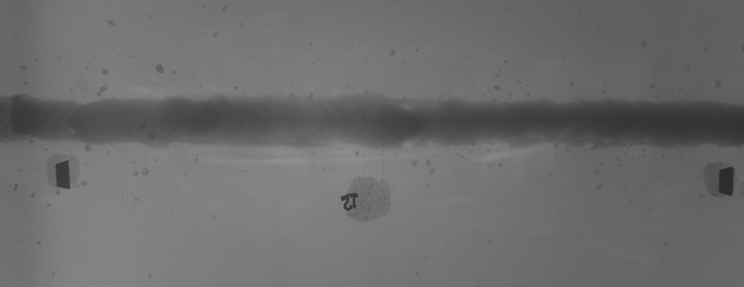
I got here a rather interesting project: on radiographs of welds to find wire samples of standard sizes. It would seem, how much has already been written about the search patterns in the image, developed standard approaches and techniques, but when it comes to real-world problems, academic methods are not as effective as expected from them. For starters, try finding all seven wires here:
')
In fact, this is not the easiest shot, but in the end even everything was found on it:

So, what conditions were announced to me:
- files will be tiff and can be quite large - more than 200 MB
- images can be both positive and negative
- on one picture there can be several standards, it is necessary to find everything
- samples lie either almost vertically (+ -10 degrees) or almost horizontally
- frames may have other standards and other elements
- seams can be both straight and elliptical, horizontal and vertical
- the sample may lie on or near the seam
Maximum time to search for standards in the picture:
- 3 seconds for a picture smaller than 100 MB
- 5 seconds for a snapshot more than 100 MB and less than 200 MB
- 10 seconds, for a picture larger than 200 MB.
I was also given GOST standards of two types of standards that looked something like this:

Those. Each standard consists of 7 wires of a certain length and a decreasing diameter located at predetermined distances.
Lengths are different: 10, 20, 25, 50 mm.
For each length there is a set of standards with different wire thicknesses, for example, one standard with 25 mm wire length has wire diameters of 3.2mm, 2.5mm, 2mm, 1.6mm, 1.25mm, 1.0mm, 0.8mm, 0.63mm, and the other - 1.0 mm, 0.8mm, 0.63mm, 0.5mm, 0.4mm, 0.32mm, 0.25mm.
In total, there were about 16 standards.
Thus, I had to localize fully deterministic objects in images of different quality.
I immediately thought about using trained classifiers, but I was embarrassed by the fact that I had only 82 files with different standards, and for normal training of the classifier, we still need thousands of images. So this way had to be swept away immediately.
The task of searching for linear segments is itself well reflected in the literature.
The very first thing that comes to mind is to look for segments of the Hough transformation, but, firstly, it is very resource-intensive, and secondly, weak signals among the stronger ones after the transformation will not look any easier. Even if you take a pretty good framing:

it is still rather difficult to find delays:

(this is how it should look like: ->
->  )
)
Another option would be to use filtering circuits, but the problem arises: how to choose the binarization threshold in automatic mode?
Yes, and what to do with the contours, which mainly choose the weld or something else?
-> 


Loop detector with different binarization levels
The same applies to other beamlet type detectors .
As it turned out, a very productive step was the simple calculation of the gradient map, i.e. just calculating the difference between two adjacent pixels. Such a step sharply highlights the sharp edges and almost erases all the slow transitions. Here's what, for example, happened after applying gradients twice:
It was:

has become:

Contrast is enhanced on the bottom image for clarity.
Agree, even with the naked eye it became much easier to find the wires.
Immediately, another problem became visible - noise. And the noise level is uneven in the picture.
How can we highlight areas of interest for a more detailed study? Some method is needed that would take into account the local noise level and detect emissions that significantly exceed the average deviation.
Since all the geometry of the standards is known to us in advance, we can choose the size of the window in which the local statistics will be collected, thus we will be able to automate the choice of the binarization threshold. Moreover, since we know in advance that the wires will be approximately vertically, I decided to make an additional filter: if in the selected window significant emissions are more than 1/2 of the vertical size of the window, then we select the entire vertical bar as an area of interest for further analysis ( looking ahead, I’ll say that I also added an additional statistical detector for emissions, which are several times higher than the standard deviation - it was necessary that all letters and numbers on the frame also fall entirely into the field of further analysis and where they could be filtered out. Without it, a lot of false positives were due to partial areas to find letters and numbers).
Here is what happened at this stage:

Here, the resulting areas of interest are indicated in blue, pink, and black. The current cluster for which recognition is performed is highlighted in pink.
We coped with the preprocessing, we must go directly to the recognition of standards.
The first step is clustering. It is necessary to somehow break all the found points into clusters in order to work with them later.
Here, the option to add all new points to the current cluster came up pretty well, if they are located + -2 pixels vertically / horizontally.
In principle, this method can fail if the weld breaks the wire into two separated regions, so a second clustering option was provided, when +15 points were viewed vertically.
Here again, different options are possible.
Since the clusters are already allocated, it would be possible to take them and try to enter the calculated versions of the standards with different angles, scales, shifts into the original picture ... But as it turned out, this is again quite laborious and you can invent a bicycle.
Namely: since we have almost vertical stripes, let's just make a projection along them, not even of the original picture or gradient maps, but of the clusters found. This turned out to be enough to determine which particular reference is on the image, if there are clusters that correspond to at least three wires.
Actually, I tried to make projections both on the original picture and on the gradient map, but there the noise was quite strong, and since we had already successfully dealt with it when searching for clusters, we can simply use the results obtained.
All this led to the following algorithm:
1. for each reference, we check that the cluster length approximately corresponds to the length of the reference wires.
2. we take a cluster, we consider the projection along it + -100-150 pixels on the right and on the left, we have one-dimensional! array with peaks in places of the found clusters.
The fact that the one-dimensional array immediately gives us a performance gain, plus there is no need to look for corners (parallel wires).
3. for several close scales (we know the scale only approximately), we calculate how the similar projection of each reference will look and make a convolution of the obtained projection of the reference and projections along the cluster + we consider how many peaks in the projection along the cluster are.
4. if there are other clusters on both sides of the cluster - we are in the middle of the standard, go to the next cluster
5. if nothing is detected from both sides - we most likely stumbled upon a false cluster formed by “artifacts”
6. If there is nothing on one side, and less than two peaks on the other, these are either artifacts or the wires are too thin, in any case, we will not be able to establish exactly where our standard is rotated only by two wires.
7. if on the one hand there are more than 2 peaks, we check that the convolution with the reference projection gives a tangible contribution.
convolution itself was considered so:
where WSKernel is the reference projection, which has 1 in places where there is a wire and -1 where it does not exist (that is, it looks like 1,1,1,1,1,1, -1, -1, -1, -1 1,1,1, ...)
ltrtr is the projection itself along the cluster
tracemax is the maximum intensity of the projection along the cluster
All this works so that in places where there is a peak and it coincides with the standard to make a positive contribution (-k * tracemax is needed to penalize not finding a wire in the right place, k = 0.1 turned out to be the most productive), and where it is, but not matches - negative.
After passing through several scales and standards, the maximum contribution is selected and it is considered that this cluster corresponds to this standard with the calculated scale factor.
Further - only drawing and delivery of results.
Well, a couple of examples:


')
In fact, this is not the easiest shot, but in the end even everything was found on it:
So, what conditions were announced to me:
- files will be tiff and can be quite large - more than 200 MB
- images can be both positive and negative
- on one picture there can be several standards, it is necessary to find everything
- samples lie either almost vertically (+ -10 degrees) or almost horizontally
- frames may have other standards and other elements
- seams can be both straight and elliptical, horizontal and vertical
- the sample may lie on or near the seam
Maximum time to search for standards in the picture:
- 3 seconds for a picture smaller than 100 MB
- 5 seconds for a snapshot more than 100 MB and less than 200 MB
- 10 seconds, for a picture larger than 200 MB.
I was also given GOST standards of two types of standards that looked something like this:
Those. Each standard consists of 7 wires of a certain length and a decreasing diameter located at predetermined distances.
Lengths are different: 10, 20, 25, 50 mm.
For each length there is a set of standards with different wire thicknesses, for example, one standard with 25 mm wire length has wire diameters of 3.2mm, 2.5mm, 2mm, 1.6mm, 1.25mm, 1.0mm, 0.8mm, 0.63mm, and the other - 1.0 mm, 0.8mm, 0.63mm, 0.5mm, 0.4mm, 0.32mm, 0.25mm.
In total, there were about 16 standards.
Thus, I had to localize fully deterministic objects in images of different quality.
Choosing a path
I immediately thought about using trained classifiers, but I was embarrassed by the fact that I had only 82 files with different standards, and for normal training of the classifier, we still need thousands of images. So this way had to be swept away immediately.
The task of searching for linear segments is itself well reflected in the literature.
The very first thing that comes to mind is to look for segments of the Hough transformation, but, firstly, it is very resource-intensive, and secondly, weak signals among the stronger ones after the transformation will not look any easier. Even if you take a pretty good framing:
it is still rather difficult to find delays:
(this is how it should look like:
-> )Another option would be to use filtering circuits, but the problem arises: how to choose the binarization threshold in automatic mode?
Yes, and what to do with the contours, which mainly choose the weld or something else?
-> Loop detector with different binarization levels
The same applies to other beamlet type detectors .
What can be done to improve the situation?
As it turned out, a very productive step was the simple calculation of the gradient map, i.e. just calculating the difference between two adjacent pixels. Such a step sharply highlights the sharp edges and almost erases all the slow transitions. Here's what, for example, happened after applying gradients twice:
It was:
has become:
Contrast is enhanced on the bottom image for clarity.
Agree, even with the naked eye it became much easier to find the wires.
Immediately, another problem became visible - noise. And the noise level is uneven in the picture.
How can we highlight areas of interest for a more detailed study? Some method is needed that would take into account the local noise level and detect emissions that significantly exceed the average deviation.
Since all the geometry of the standards is known to us in advance, we can choose the size of the window in which the local statistics will be collected, thus we will be able to automate the choice of the binarization threshold. Moreover, since we know in advance that the wires will be approximately vertically, I decided to make an additional filter: if in the selected window significant emissions are more than 1/2 of the vertical size of the window, then we select the entire vertical bar as an area of interest for further analysis ( looking ahead, I’ll say that I also added an additional statistical detector for emissions, which are several times higher than the standard deviation - it was necessary that all letters and numbers on the frame also fall entirely into the field of further analysis and where they could be filtered out. Without it, a lot of false positives were due to partial areas to find letters and numbers).
Here is what happened at this stage:
Here, the resulting areas of interest are indicated in blue, pink, and black. The current cluster for which recognition is performed is highlighted in pink.
We coped with the preprocessing, we must go directly to the recognition of standards.
The first step is clustering. It is necessary to somehow break all the found points into clusters in order to work with them later.
Here, the option to add all new points to the current cluster came up pretty well, if they are located + -2 pixels vertically / horizontally.
In principle, this method can fail if the weld breaks the wire into two separated regions, so a second clustering option was provided, when +15 points were viewed vertically.
Pattern Recognition
Here again, different options are possible.
Since the clusters are already allocated, it would be possible to take them and try to enter the calculated versions of the standards with different angles, scales, shifts into the original picture ... But as it turned out, this is again quite laborious and you can invent a bicycle.
Namely: since we have almost vertical stripes, let's just make a projection along them, not even of the original picture or gradient maps, but of the clusters found. This turned out to be enough to determine which particular reference is on the image, if there are clusters that correspond to at least three wires.
Actually, I tried to make projections both on the original picture and on the gradient map, but there the noise was quite strong, and since we had already successfully dealt with it when searching for clusters, we can simply use the results obtained.
All this led to the following algorithm:
1. for each reference, we check that the cluster length approximately corresponds to the length of the reference wires.
2. we take a cluster, we consider the projection along it + -100-150 pixels on the right and on the left, we have one-dimensional! array with peaks in places of the found clusters.
The fact that the one-dimensional array immediately gives us a performance gain, plus there is no need to look for corners (parallel wires).
3. for several close scales (we know the scale only approximately), we calculate how the similar projection of each reference will look and make a convolution of the obtained projection of the reference and projections along the cluster + we consider how many peaks in the projection along the cluster are.
4. if there are other clusters on both sides of the cluster - we are in the middle of the standard, go to the next cluster
5. if nothing is detected from both sides - we most likely stumbled upon a false cluster formed by “artifacts”
6. If there is nothing on one side, and less than two peaks on the other, these are either artifacts or the wires are too thin, in any case, we will not be able to establish exactly where our standard is rotated only by two wires.
7. if on the one hand there are more than 2 peaks, we check that the convolution with the reference projection gives a tangible contribution.
convolution itself was considered so:
if (WSKernel[i] == 1) { // punish more if there is no line: convlft += WSKernel[i] * (ltrtr[lngth - i] - k * tracemax); //ltrtr is always positive as a sum of presences of clusters convrgt += WSKernel[i] * (ltrtr[lngth + i] - k * tracemax); } else // WSKernel[[i]]==-1 { convlft += WSKernel[i] * ltrtr[lngth - i]; convrgt += WSKernel[i] * ltrtr[lngth + i]; } where WSKernel is the reference projection, which has 1 in places where there is a wire and -1 where it does not exist (that is, it looks like 1,1,1,1,1,1, -1, -1, -1, -1 1,1,1, ...)
ltrtr is the projection itself along the cluster
tracemax is the maximum intensity of the projection along the cluster
All this works so that in places where there is a peak and it coincides with the standard to make a positive contribution (-k * tracemax is needed to penalize not finding a wire in the right place, k = 0.1 turned out to be the most productive), and where it is, but not matches - negative.
After passing through several scales and standards, the maximum contribution is selected and it is considered that this cluster corresponds to this standard with the calculated scale factor.
Further - only drawing and delivery of results.
Well, a couple of examples:
Source: https://habr.com/ru/post/236309/
All Articles