Lossless Data Compression Algorithms, Part 2
Part 1
For data compression, many techniques are invented. Most of them combine several compression principles to create a complete algorithm. Even good principles, when combined together, give the best result. Most technicians use the principle of entropy coding, but others are often found - Run-Length Encoding and Burrows-Wheeler Transform.
This is a very simple algorithm. It replaces a series of two or more identical characters with a number indicating the length of the series, followed by the character itself. Useful for highly redundant data, such as images with a large number of identical pixels, or in combination with algorithms such as BWT.
A simple example:
')
At the entrance: AAABBCCCCDEEEEEEAAAAAAAAAAAAAAAAAAAAAAAAAAAAAAAAAAAAAA
Output: 3A2B4C1D6E38A
The algorithm, invented in 1994, reversibly transforms a block of data so as to maximize the repetition of the same characters. It itself does not compress the data, but prepares them for more efficient compression through RLE or another compression algorithm.
Algorithm:
- create an array of strings
- create all possible transformations of the incoming data line, each of which is stored in an array
- sort the array
- return the last column
The algorithm works best with big data with lots of duplicate characters. An example of working on a suitable data array (& denotes the end of the file)
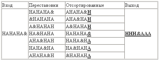
Due to the alternation of identical symbols, the output of the algorithm is optimal for compressing RLE, which gives “3H & 3A”. But on real data, unfortunately, such optimal results usually do not work.
Entropy in this case means the minimum number of bits needed on average to represent a character. Simple EC combines the statistical model and the encoder itself. The input file is parsed to build a statistical model consisting of the probabilities of the occurrence of certain characters. Then the encoder, using the model, determines which bit or byte encodings to assign to each character so that the most common ones are represented by the shortest encodings, and vice versa.
One of the earliest techniques (1949). Creates a binary tree to represent the probabilities of the occurrence of each of the characters. Then they are sorted so that the most common ones are at the top of the tree, and vice versa.
The code for the symbol is obtained by searching the tree, and adding 0 or 1, depending on whether we go left or right. For example, the path to “A” is two branches to the left and one to the right, its code will be “110”. The algorithm does not always give optimal codes due to the method of constructing the tree from the bottom up. Therefore, the Huffman algorithm is now used, suitable for any input data.
1. parsim input, count the number of occurrences of all characters
2. determine the probability of occurrence of each of them
3. sort the characters by the probability of occurrence
4. we divide the list in half so that the sum of the probabilities in the left branch is approximately equal to the sum in the right
5. add 0 or 1 for the left and right nodes, respectively
6. repeat steps 4 and 5 for the right and left subtrees until each node is a “sheet”
This is a variant of entropy coding, which works by a method similar to the previous algorithm, but the binary tree is built from top to bottom in order to achieve an optimal result.
1. Parsing input, count the number of repetitions of characters.
2. Determine the probability of occurrence of each character.
3. Sort the list by probabilities (the most frequent at the beginning)
4. Create sheets for each character, and add them to the queue
5. while the queue consists of more than one character:
- take from the queue two sheets with the least probabilities
- to the code of the first we add 0, to the code of the second - 1
- create a node with a probability equal to the sum of the probabilities of two nodes
- we hang the first node on the left side, the second - on the right side
- add the resulting node to the queue
6. The last node in the queue will be the root of the binary tree.
It was developed in 1979 by IBM for use in their mainframes. It achieves a very good degree of compression, usually greater than that of Huffman, but it is relatively complex compared to previous ones.
Instead of splitting the probabilities into a tree, the algorithm converts the input data into one rational number from 0 to 1.
In general, the algorithm is as follows:
1. count the number of unique characters at the entrance. This number will represent the basis for the calculation of b (b = 2 - binary, etc.).
2. calculate the total length of the input
3. assign “codes” from 0 to b to each of the unique characters in the order they appear
4. replace characters with codes, getting a number in the number system with base b
5. convert the resulting number to binary
Example. At the input line "ABCDAABD"
1. 4 unique characters, base = 4, data length = 8
2. assign codes: A = 0, B = 1, C = 2, D = 3
3. we get the number “0.01230013”
4. convert the “0.01231123” from the quaternary to the binary system: 0.01101100000111
If we assume that we are dealing with eight-bit characters, then we have 8x8 = 64 bits at the input, and 15 at the output, that is, the compression ratio is 24%.
It all started with the algorithm LZ77 (1977), which introduced a new concept of a “sliding window”, which made it possible to significantly improve data compression. LZ77 uses a dictionary containing data triples - offset, run length and discrepancy symbol. Offset - how far from the beginning of the file is the phrase. The length of the series - how many characters, counting from the offset, belong to the phrase. The divergence symbol indicates that a new phrase has been found, similar to the one indicated by offset and length, with the exception of this symbol. The dictionary changes as the file is parsed using a sliding window. For example, the window size may be 64 MB, then the dictionary will contain data from the last 64 megabytes of input data.
For example, for the input data "abbadabba" the result will be "abb (0,1, 'd') (0,3, 'a')"
In this case, the result was longer than the input, but it usually turns out to be shorter.
A modification of the LZ77 algorithm proposed by Michael Road in 1981. Unlike the LZ77, it works in linear time, but it requires more memory. Usually loses LZ78 in compression.
Coined by Phil Katz in 1993, and is used in most modern archivers. Is a combination of LZ77 or LZSS with Huffman coding.
Patented variation DEFLATE with increasing dictionary up to 64 KB. Squeezes better and faster, but not used everywhere, because is not open.
The Lempel-Ziva-Storer-Cymansky algorithm was introduced in 1982. An improved version of LZ77, which calculates whether the size of the result will not increase the replacement of the original data with coded data.
It is still used in popular archivers, for example RAR. Sometimes - to compress data during transmission over the network.
It was developed in 1987, stands for Lempel-Ziv-Huffman. Variation LZSS, uses Huffman coding to compress pointers. Squeezes a little better, but significantly slower.
Developed in 1987 by Timothy Bell, as an option LZSS. Like LZH, LZB reduces the resulting file size by efficiently encoding pointers. This is achieved by gradually increasing the size of the pointers while increasing the size of the sliding window. Compression is higher than that of LZSS and LZH, but the speed is much less.
It stands for “Lempel-Ziv with a reduced offset”, improves the LZ77 algorithm, reducing the offset to reduce the amount of data needed to encode an offset-length pair. It was first introduced in 1991 in the LZRW4 algorithm from Ross Williams. Other variations are BALZ, QUAD, and RZM. The well-optimized ROLZ achieves almost the same compression ratios as the LZMA - but it has not gained popularity.
"Lempel-Ziv with a prediction." Variation of ROLZ with offset = 1. There are several options, some focused on the speed of compression, others on the degree. The LZW4 algorithm uses arithmetic coding for best compression.
The algorithm from Ron Williams of 1991, where he first introduced the concept of reducing bias. Reaches high degrees of compression at a decent speed. Then Williams made variations of LZRW1-A, 2, 3, 3-A, and 4
A variant from Jeff Bonvik (hence the “JB”) from 1998, for use in the Solaris Z File System (ZFS) file system. A variant of the LZRW1 algorithm, reworked for high speeds, as required by the use of file operations and speed of disk operations.
Lempel-Ziv-Stac, developed at Stac Electronics in 1994 for use in disk compression programs. A modification of the LZ77, distinguishing between characters and length-offset pairs, in addition to removing the next character encountered. Very similar to LZSS.
It was developed in 1995 by J. Forbes and T.Potanen for the Amiga. Forbes sold the algorithm to Microsoft in 1996, and settled there to work on it, with the result that its improved version was used in the files CAB, CHM, WIM and Xbox Live Avatars.
Developed in 1996 by Markus Oberhümer with a view to the speed of compression and decompression. Allows you to adjust the levels of compression, consumes very little memory. Looks like a lzss.
“Lempel-Ziv Markov chain Algorithm”, appeared in 1998 in the 7-zip archiver, which demonstrated compression better than almost all archivers. The algorithm uses a chain of compression methods to achieve the best result. Initially, the slightly modified LZ77, which works at the bit level (as opposed to the usual method of working with bytes), parses the data. Its output is subjected to arithmetic coding. Then other algorithms can be applied. The result is the best compression among all archivers.
The next version of LZMA, from 2009, uses multithreading and stores incompressible data a little more efficiently.
The concept, created in 2001, proposes a statistical analysis of data in combination with the LZ77 to optimize the codes stored in the dictionary.
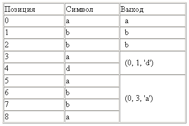
Algorithm of 1978, authors - Lempel and Ziv. Instead of using a sliding window to create a dictionary, a dictionary is compiled when parsing data from a file. Dictionary size is usually measured in several megabytes. Differences in variants of this algorithm are based on what to do when the dictionary is full.
When parsing a file, the algorithm adds each new character or their combination to the dictionary. For each character at the input, a dictionary form (index + unknown character) is created at the output. If the first character of a string is already in the dictionary, look for the substrings of the given string in the dictionary, and the longest one is used to build the index. The data pointed to by the index is added to the last character of the unknown substring. If the current character is not found, the index is set to 0, indicating that this is a single character entry in the dictionary. Entries form a linked list.
The input data "abbadabbaabaad" at the output will give "(0, a) (0, b) (2, a) (0, d) (1, b) (3, a) (6, d)"
An input such as "abbadabbaabaad" would generate the output "(0, a) (0, b) (2, a) (0, d) (1, b) (3, a) (6, d)". It can be seen in the following example:
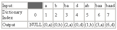
Lempel-Ziv-Welch, 1984. The most popular version of the LZ78, despite the patented. The algorithm gets rid of extra characters on the output and the data consists only of pointers. It also saves all dictionary characters before compression and uses other tricks to improve compression — for example, encoding the last character of the previous phrase as the first character of the next. Used in GIF, early versions of ZIP and other special applications. Very fast, but loses in compression to newer algorithms.
Lempel-Ziv Compression. LZW modification used in UNIX utilities. It monitors the degree of compression, and as soon as it exceeds the specified limit, the dictionary is redone again.
Lempel-Ziv-Tischer. When the dictionary is filled, deletes the less frequently used phrases and replaces them with new ones. Not gained popularity.
Victor Miller and Mark Wegman, 1984. Acts as LZT, but combines not the similar data in the dictionary, but the last two phrases. As a result, the dictionary grows faster, and you often have to get rid of rarely used phrases. Also unpopular.
James Storer, 1988. Modification of LZMW. “AP” means “all prefixes” - instead of saving one phrase at each iteration, each change is saved in the dictionary. For example, if the last phrase was “last” and the current phrase was “next”, then in the dictionary there are “lastn”, “lastne”, “lastnex”, “lastnext”.
LZW version of 2006, working with combinations of characters, rather than with individual characters. Works successfully with data sets that have frequently repeated combinations of characters, such as XML. Typically used with a preprocessor that breaks data into combinations.
1985, Matti Jacobson. One of the few options LZ78, different from LZW. Saves each unique line in already processed input data, and assigns unique codes to all of them. When filling out the dictionary, single entries are removed from it.
Partial prediction - uses already processed data to predict which character will be next in sequence, thus reducing the entropy of the output. Usually combined with arithmetic encoder or adaptive Huffman coding. PPMd variation used in rar and 7-zip
An open source implementation of BWT. With ease of implementation achieves a good compromise between speed and compression ratio, and therefore is popular in UNIX. First, data is processed using RLE, then BWT, then the data is sorted in a special way to get long sequences of identical characters, after which RLE is applied to it again. And finally, the Huffman Encoder ends the process.
Matt Mahone, 2002. Improved PPM (d). Improves them with the help of an interesting technique called “context mixing” (context mixing). In this technique, several predictive algorithms are combined to improve the prediction of the next character. Now it is one of the most promising algorithms. Since its first implementation, two dozen options have been created, some of which set compression records. Minus - a small speed due to the need to use several models. The variant called PAQ80 supports 64 bits and shows a serious improvement in the speed of work (used, in particular, in the PeaZip program for Windows).
Data Compression Techniques
For data compression, many techniques are invented. Most of them combine several compression principles to create a complete algorithm. Even good principles, when combined together, give the best result. Most technicians use the principle of entropy coding, but others are often found - Run-Length Encoding and Burrows-Wheeler Transform.
Series Length Coding (RLE)
This is a very simple algorithm. It replaces a series of two or more identical characters with a number indicating the length of the series, followed by the character itself. Useful for highly redundant data, such as images with a large number of identical pixels, or in combination with algorithms such as BWT.
A simple example:
')
At the entrance: AAABBCCCCDEEEEEEAAAAAAAAAAAAAAAAAAAAAAAAAAAAAAAAAAAAAA
Output: 3A2B4C1D6E38A
Burrows-Wheeler Transformation (BWT)
The algorithm, invented in 1994, reversibly transforms a block of data so as to maximize the repetition of the same characters. It itself does not compress the data, but prepares them for more efficient compression through RLE or another compression algorithm.
Algorithm:
- create an array of strings
- create all possible transformations of the incoming data line, each of which is stored in an array
- sort the array
- return the last column
The algorithm works best with big data with lots of duplicate characters. An example of working on a suitable data array (& denotes the end of the file)
Due to the alternation of identical symbols, the output of the algorithm is optimal for compressing RLE, which gives “3H & 3A”. But on real data, unfortunately, such optimal results usually do not work.
Entropy coding
Entropy in this case means the minimum number of bits needed on average to represent a character. Simple EC combines the statistical model and the encoder itself. The input file is parsed to build a statistical model consisting of the probabilities of the occurrence of certain characters. Then the encoder, using the model, determines which bit or byte encodings to assign to each character so that the most common ones are represented by the shortest encodings, and vice versa.
Shannon-Fano Algorithm
One of the earliest techniques (1949). Creates a binary tree to represent the probabilities of the occurrence of each of the characters. Then they are sorted so that the most common ones are at the top of the tree, and vice versa.
The code for the symbol is obtained by searching the tree, and adding 0 or 1, depending on whether we go left or right. For example, the path to “A” is two branches to the left and one to the right, its code will be “110”. The algorithm does not always give optimal codes due to the method of constructing the tree from the bottom up. Therefore, the Huffman algorithm is now used, suitable for any input data.
1. parsim input, count the number of occurrences of all characters
2. determine the probability of occurrence of each of them
3. sort the characters by the probability of occurrence
4. we divide the list in half so that the sum of the probabilities in the left branch is approximately equal to the sum in the right
5. add 0 or 1 for the left and right nodes, respectively
6. repeat steps 4 and 5 for the right and left subtrees until each node is a “sheet”
Huffman coding
This is a variant of entropy coding, which works by a method similar to the previous algorithm, but the binary tree is built from top to bottom in order to achieve an optimal result.
1. Parsing input, count the number of repetitions of characters.
2. Determine the probability of occurrence of each character.
3. Sort the list by probabilities (the most frequent at the beginning)
4. Create sheets for each character, and add them to the queue
5. while the queue consists of more than one character:
- take from the queue two sheets with the least probabilities
- to the code of the first we add 0, to the code of the second - 1
- create a node with a probability equal to the sum of the probabilities of two nodes
- we hang the first node on the left side, the second - on the right side
- add the resulting node to the queue
6. The last node in the queue will be the root of the binary tree.
Arithmetic coding
It was developed in 1979 by IBM for use in their mainframes. It achieves a very good degree of compression, usually greater than that of Huffman, but it is relatively complex compared to previous ones.
Instead of splitting the probabilities into a tree, the algorithm converts the input data into one rational number from 0 to 1.
In general, the algorithm is as follows:
1. count the number of unique characters at the entrance. This number will represent the basis for the calculation of b (b = 2 - binary, etc.).
2. calculate the total length of the input
3. assign “codes” from 0 to b to each of the unique characters in the order they appear
4. replace characters with codes, getting a number in the number system with base b
5. convert the resulting number to binary
Example. At the input line "ABCDAABD"
1. 4 unique characters, base = 4, data length = 8
2. assign codes: A = 0, B = 1, C = 2, D = 3
3. we get the number “0.01230013”
4. convert the “0.01231123” from the quaternary to the binary system: 0.01101100000111
If we assume that we are dealing with eight-bit characters, then we have 8x8 = 64 bits at the input, and 15 at the output, that is, the compression ratio is 24%.
Algorithm classification
Algorithms using the “sliding window” method
It all started with the algorithm LZ77 (1977), which introduced a new concept of a “sliding window”, which made it possible to significantly improve data compression. LZ77 uses a dictionary containing data triples - offset, run length and discrepancy symbol. Offset - how far from the beginning of the file is the phrase. The length of the series - how many characters, counting from the offset, belong to the phrase. The divergence symbol indicates that a new phrase has been found, similar to the one indicated by offset and length, with the exception of this symbol. The dictionary changes as the file is parsed using a sliding window. For example, the window size may be 64 MB, then the dictionary will contain data from the last 64 megabytes of input data.
For example, for the input data "abbadabba" the result will be "abb (0,1, 'd') (0,3, 'a')"
In this case, the result was longer than the input, but it usually turns out to be shorter.
Lzr
A modification of the LZ77 algorithm proposed by Michael Road in 1981. Unlike the LZ77, it works in linear time, but it requires more memory. Usually loses LZ78 in compression.
Deflate
Coined by Phil Katz in 1993, and is used in most modern archivers. Is a combination of LZ77 or LZSS with Huffman coding.
DEFLATE64
Patented variation DEFLATE with increasing dictionary up to 64 KB. Squeezes better and faster, but not used everywhere, because is not open.
Lzss
The Lempel-Ziva-Storer-Cymansky algorithm was introduced in 1982. An improved version of LZ77, which calculates whether the size of the result will not increase the replacement of the original data with coded data.
It is still used in popular archivers, for example RAR. Sometimes - to compress data during transmission over the network.
Lzh
It was developed in 1987, stands for Lempel-Ziv-Huffman. Variation LZSS, uses Huffman coding to compress pointers. Squeezes a little better, but significantly slower.
Lzb
Developed in 1987 by Timothy Bell, as an option LZSS. Like LZH, LZB reduces the resulting file size by efficiently encoding pointers. This is achieved by gradually increasing the size of the pointers while increasing the size of the sliding window. Compression is higher than that of LZSS and LZH, but the speed is much less.
Rolz
It stands for “Lempel-Ziv with a reduced offset”, improves the LZ77 algorithm, reducing the offset to reduce the amount of data needed to encode an offset-length pair. It was first introduced in 1991 in the LZRW4 algorithm from Ross Williams. Other variations are BALZ, QUAD, and RZM. The well-optimized ROLZ achieves almost the same compression ratios as the LZMA - but it has not gained popularity.
Lzp
"Lempel-Ziv with a prediction." Variation of ROLZ with offset = 1. There are several options, some focused on the speed of compression, others on the degree. The LZW4 algorithm uses arithmetic coding for best compression.
Lzrw1
The algorithm from Ron Williams of 1991, where he first introduced the concept of reducing bias. Reaches high degrees of compression at a decent speed. Then Williams made variations of LZRW1-A, 2, 3, 3-A, and 4
Lzjb
A variant from Jeff Bonvik (hence the “JB”) from 1998, for use in the Solaris Z File System (ZFS) file system. A variant of the LZRW1 algorithm, reworked for high speeds, as required by the use of file operations and speed of disk operations.
Lzs
Lempel-Ziv-Stac, developed at Stac Electronics in 1994 for use in disk compression programs. A modification of the LZ77, distinguishing between characters and length-offset pairs, in addition to removing the next character encountered. Very similar to LZSS.
Lzx
It was developed in 1995 by J. Forbes and T.Potanen for the Amiga. Forbes sold the algorithm to Microsoft in 1996, and settled there to work on it, with the result that its improved version was used in the files CAB, CHM, WIM and Xbox Live Avatars.
Lzo
Developed in 1996 by Markus Oberhümer with a view to the speed of compression and decompression. Allows you to adjust the levels of compression, consumes very little memory. Looks like a lzss.
Lzma
“Lempel-Ziv Markov chain Algorithm”, appeared in 1998 in the 7-zip archiver, which demonstrated compression better than almost all archivers. The algorithm uses a chain of compression methods to achieve the best result. Initially, the slightly modified LZ77, which works at the bit level (as opposed to the usual method of working with bytes), parses the data. Its output is subjected to arithmetic coding. Then other algorithms can be applied. The result is the best compression among all archivers.
Lzma2
The next version of LZMA, from 2009, uses multithreading and stores incompressible data a little more efficiently.
Lempel-Ziv statistical algorithm
The concept, created in 2001, proposes a statistical analysis of data in combination with the LZ77 to optimize the codes stored in the dictionary.
Algorithms using the dictionary
Lz78
Algorithm of 1978, authors - Lempel and Ziv. Instead of using a sliding window to create a dictionary, a dictionary is compiled when parsing data from a file. Dictionary size is usually measured in several megabytes. Differences in variants of this algorithm are based on what to do when the dictionary is full.
When parsing a file, the algorithm adds each new character or their combination to the dictionary. For each character at the input, a dictionary form (index + unknown character) is created at the output. If the first character of a string is already in the dictionary, look for the substrings of the given string in the dictionary, and the longest one is used to build the index. The data pointed to by the index is added to the last character of the unknown substring. If the current character is not found, the index is set to 0, indicating that this is a single character entry in the dictionary. Entries form a linked list.
The input data "abbadabbaabaad" at the output will give "(0, a) (0, b) (2, a) (0, d) (1, b) (3, a) (6, d)"
An input such as "abbadabbaabaad" would generate the output "(0, a) (0, b) (2, a) (0, d) (1, b) (3, a) (6, d)". It can be seen in the following example:
Lzw
Lempel-Ziv-Welch, 1984. The most popular version of the LZ78, despite the patented. The algorithm gets rid of extra characters on the output and the data consists only of pointers. It also saves all dictionary characters before compression and uses other tricks to improve compression — for example, encoding the last character of the previous phrase as the first character of the next. Used in GIF, early versions of ZIP and other special applications. Very fast, but loses in compression to newer algorithms.
Lzc
Lempel-Ziv Compression. LZW modification used in UNIX utilities. It monitors the degree of compression, and as soon as it exceeds the specified limit, the dictionary is redone again.
Lzt
Lempel-Ziv-Tischer. When the dictionary is filled, deletes the less frequently used phrases and replaces them with new ones. Not gained popularity.
Lzmw
Victor Miller and Mark Wegman, 1984. Acts as LZT, but combines not the similar data in the dictionary, but the last two phrases. As a result, the dictionary grows faster, and you often have to get rid of rarely used phrases. Also unpopular.
Lzap
James Storer, 1988. Modification of LZMW. “AP” means “all prefixes” - instead of saving one phrase at each iteration, each change is saved in the dictionary. For example, if the last phrase was “last” and the current phrase was “next”, then in the dictionary there are “lastn”, “lastne”, “lastnex”, “lastnext”.
Lzwl
LZW version of 2006, working with combinations of characters, rather than with individual characters. Works successfully with data sets that have frequently repeated combinations of characters, such as XML. Typically used with a preprocessor that breaks data into combinations.
Lzj
1985, Matti Jacobson. One of the few options LZ78, different from LZW. Saves each unique line in already processed input data, and assigns unique codes to all of them. When filling out the dictionary, single entries are removed from it.
Algorithms that do not use a dictionary
PPM
Partial prediction - uses already processed data to predict which character will be next in sequence, thus reducing the entropy of the output. Usually combined with arithmetic encoder or adaptive Huffman coding. PPMd variation used in rar and 7-zip
bzip2
An open source implementation of BWT. With ease of implementation achieves a good compromise between speed and compression ratio, and therefore is popular in UNIX. First, data is processed using RLE, then BWT, then the data is sorted in a special way to get long sequences of identical characters, after which RLE is applied to it again. And finally, the Huffman Encoder ends the process.
PAQ
Matt Mahone, 2002. Improved PPM (d). Improves them with the help of an interesting technique called “context mixing” (context mixing). In this technique, several predictive algorithms are combined to improve the prediction of the next character. Now it is one of the most promising algorithms. Since its first implementation, two dozen options have been created, some of which set compression records. Minus - a small speed due to the need to use several models. The variant called PAQ80 supports 64 bits and shows a serious improvement in the speed of work (used, in particular, in the PeaZip program for Windows).
Source: https://habr.com/ru/post/235553/
All Articles