The use of machine learning in trading
Translator’s note 1. I came across this blog in one of the machine learning reviews. If you are well versed in machine learning, then in this article you will not find anything interesting for yourself. It is quite superficial and affects only the basics. If you, like me, are just starting to be interested in this topic, then welcome under cat.
Translator's note 2. The code will be small, but the one that is written in R, but do not despair if you have never seen it before. Before this article, I also did not know anything about it, so I specifically wrote a “spur” for the language, including everything that you will find in the article. If you want to figure it out for yourself, I recommend starting with a small course on CodeSchool . On Habré there is also interesting information and useful links . And finally , here is a big cheat sheet.
Translator's note 3. Article from two parts, however the most interesting begins only in the second part, therefore I have allowed myself to unite them in one article.

In this series of articles, I am going to build and test a simple asset management strategy based on machine learning step by step. The first part will be devoted to the basic concepts of machine learning and their application to the financial markets.
Machine learning is one of the most promising areas in financial mathematics, which in recent years has gained the reputation of a sophisticated and complex tool. In fact, everything is not so difficult.
The goal of machine learning is to build an accurate model based on historical data and then use this model for future predictions. In financial mathematics, machine learning solves the following problems:
Consider a simple example. Let's try to predict the movement of Google’s stock value one day in advance. In the next part, we will use several indicators, but now, to study the basics, we will use only one indicator: the day of the week. So let's try to predict the price movement based on the day of the week.
Below is a chart of Google stocks and a picture of the exported data from Yahoo Finance.


I added a column for the day of the week and a column for the closing price minus the opening price. Also, I added a price direction column, where I write “UP”, if the difference between the closing price and opening price is greater than 0 and “DOWN” if less:
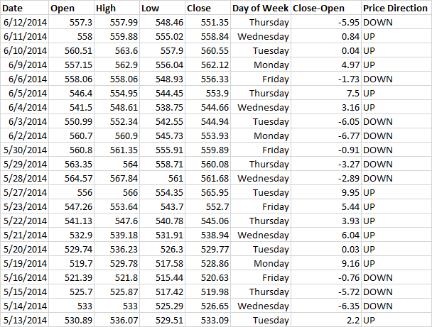
In machine learning, this data set will be called training, because the algorithm is trained on them. In other words, the algorithm scans the entire data set and establishes the relationship between the day of the week and the direction of change in the value of the stock. Note that our set is small - there are only 23 lines. In the next part, we will use hundreds of lines to build a model. In fact, the more data the better.
Now let's choose an algorithm. There are a number of algorithms that you can use, including hidden Markov Models, artificial neural networks, naive Bayes classifier, support vector machine, decision tree, analysis of variance, and many others. Here is a good list where you can understand each algorithm and understand when and which one to use. To begin, I recommend using one of the most frequently used algorithms, such as the support vector machine method or the naive Bayes classifier. Do not spend a lot of time on the choice, the most important parts of your analysis are the indicators you use and the value you predict.
')
Now that we’ve dealt with the basic concept of using machine learning algorithms in your strategy, we’ll study a simple example of using a naive Bayes classifier to predict the direction of Apple stocks. First, we will deal with how this classifier works, then we will look at a very simple example of using the day of the week to predict price movements, and at the end we will complicate the model by adding a technical indicator.
The Bayes formula allows you to find the probability that event A will happen if it is known that event B has already occurred. Usually denoted as: P (A | B).
In our example, we ask: "What is the probability that today's price will rise, if you know that today is Wednesday?". The method takes into account both the likelihood that the current price will rise based on the total number of days during which there was an increase, and based on the fact that today is Wednesday, that is, how many times the price has grown on Wednesday.
We have the opportunity to compare the likelihood that the current price will rise and the likelihood that it will fall, and use the highest value as a forecast.
So far, we have been discussing only one indicator, but as soon as there are several of them, all of mathematics quickly becomes complicated. To prevent this, a naive Bayes classifier is used ( here is a good article). It treats each indicator as independent, or not correlated (hence the naive term). Therefore, it is important to use indicators related weakly or not at all.
This is a very simplified description of the naive Bayes classifier, if you are interested in learning more about it, as well as other machine learning algorithms, see here
Now let's look at a very simple example on R. We will use the day of the week to predict the movement of Apple stock prices up or down.
First, let's make sure that we have all the libraries we need:
Now let's get the data we need:
Now that we have all the necessary data, let's get our day of the week indicator:
What we are going to predict, i.e. price movement up or down, and creating the final data set:
Now we are ready to apply the naive Bayes classifier:
Congratulations! We applied a machine learning algorithm to analyze Apple stock. Now let's look at the results.

It shows the likelihood of an increase or decrease in price based on the original data set (known as previous probabilities). We can see a small bearish bias.

Here conditional probabilities are displayed (the probability of a price rising or falling for each day of the week is indicated).
It is seen that the model is not very good, because it does not return high probabilities. Nevertheless, it is noticeable that it is better to open long positions at the beginning of the week, and short near the end.
Obviously, you will want to use a more complex strategy than just targeting the day of the week. Let's add the moving average intersection to our model (you can get more information on adding various indicators to your model here )
I prefer to use exponential moving averages, so let's look at 5-day and 10-day exponential moving averages (EMA).
First we need to calculate the EMA:
Then we calculate the intersection:
Now round up the values to 2 decimal places. This is important because if you find a value that the naive Bayes classifier did not see during the training, it will automatically calculate the probability of 0%. For example, if we look at the intersection of the EMA with an accuracy of up to 6 characters, and a high probability of price movement was found when the difference was $ 2.349181, and then a new data point was presented, which had a difference of $ 2.349182, the 0% probability of increase or lower prices. Surrounding up to 2 decimal places, we reduce the risk of encountering an unknown value for the model (provided that a sufficiently large data set was used for training, in which all the indicator values are likely to occur). This is an important limitation to keep in mind when building your own models.
Let's create a new dataset and divide the data into a training and test set. Thus, we can understand how well our model works on new data.
Now we will build a model:

The conditional probability of intersection of moving averages is a number that indicates the average value for each case ([, 1]) and for the standard deviation ([, 2]). We can see that on average, the difference between the 5-day EMA and the 10-day EMA for long and short trades was $ 0.54 and - $ 0.24, respectively.
Now we will test on new data:

A total of 164 days in the test sample. In this case, the predictions of our model coincided with real data 79 times or in 48% of cases.
This result is not good, but it should give you an idea of how to build your own machine learning strategy. In the next part, we will see how you can use this model to improve your strategy.
Translator’s note 5. Today there are 2 more articles from this series: about the decision tree and about neural networks. Articles in the same style, i.e. not deep, but only giving a general idea of the issue. If interested - I will continue to translate. About all comments, inaccuracies and other errors, write in a personal.
Translator's note 2. The code will be small, but the one that is written in R, but do not despair if you have never seen it before. Before this article, I also did not know anything about it, so I specifically wrote a “spur” for the language, including everything that you will find in the article. If you want to figure it out for yourself, I recommend starting with a small course on CodeSchool . On Habré there is also interesting information and useful links . And finally , here is a big cheat sheet.
Translator's note 3. Article from two parts, however the most interesting begins only in the second part, therefore I have allowed myself to unite them in one article.
Part 1
In this series of articles, I am going to build and test a simple asset management strategy based on machine learning step by step. The first part will be devoted to the basic concepts of machine learning and their application to the financial markets.
Machine learning is one of the most promising areas in financial mathematics, which in recent years has gained the reputation of a sophisticated and complex tool. In fact, everything is not so difficult.
The goal of machine learning is to build an accurate model based on historical data and then use this model for future predictions. In financial mathematics, machine learning solves the following problems:
- Regression. Used to predict direction and magnitude values. For example, the growth of $ 7.00 value of Google shares per day.
- Classification. Used to predict categories, such as the direction of the value of Google stock for the day.
Consider a simple example. Let's try to predict the movement of Google’s stock value one day in advance. In the next part, we will use several indicators, but now, to study the basics, we will use only one indicator: the day of the week. So let's try to predict the price movement based on the day of the week.
Below is a chart of Google stocks and a picture of the exported data from Yahoo Finance.
I added a column for the day of the week and a column for the closing price minus the opening price. Also, I added a price direction column, where I write “UP”, if the difference between the closing price and opening price is greater than 0 and “DOWN” if less:
In machine learning, this data set will be called training, because the algorithm is trained on them. In other words, the algorithm scans the entire data set and establishes the relationship between the day of the week and the direction of change in the value of the stock. Note that our set is small - there are only 23 lines. In the next part, we will use hundreds of lines to build a model. In fact, the more data the better.
Now let's choose an algorithm. There are a number of algorithms that you can use, including hidden Markov Models, artificial neural networks, naive Bayes classifier, support vector machine, decision tree, analysis of variance, and many others. Here is a good list where you can understand each algorithm and understand when and which one to use. To begin, I recommend using one of the most frequently used algorithms, such as the support vector machine method or the naive Bayes classifier. Do not spend a lot of time on the choice, the most important parts of your analysis are the indicators you use and the value you predict.
')
Part 2
Now that we’ve dealt with the basic concept of using machine learning algorithms in your strategy, we’ll study a simple example of using a naive Bayes classifier to predict the direction of Apple stocks. First, we will deal with how this classifier works, then we will look at a very simple example of using the day of the week to predict price movements, and at the end we will complicate the model by adding a technical indicator.
What is a naive Bayes classifier?
The Bayes formula allows you to find the probability that event A will happen if it is known that event B has already occurred. Usually denoted as: P (A | B).
In our example, we ask: "What is the probability that today's price will rise, if you know that today is Wednesday?". The method takes into account both the likelihood that the current price will rise based on the total number of days during which there was an increase, and based on the fact that today is Wednesday, that is, how many times the price has grown on Wednesday.
We have the opportunity to compare the likelihood that the current price will rise and the likelihood that it will fall, and use the highest value as a forecast.
So far, we have been discussing only one indicator, but as soon as there are several of them, all of mathematics quickly becomes complicated. To prevent this, a naive Bayes classifier is used ( here is a good article). It treats each indicator as independent, or not correlated (hence the naive term). Therefore, it is important to use indicators related weakly or not at all.
This is a very simplified description of the naive Bayes classifier, if you are interested in learning more about it, as well as other machine learning algorithms, see here
Step-by-Step R Example
Spur R
To work you will need:
The language itself is very simple. Script files can not be created - everything is written directly in the console.
Now, in order, all that will meet:
There is no strict typing in the language, there is no need to declare variables. To assign a value, use the sign "<-"
For example:
The vector is assigned as:
There is a special type - data frame. Visually, it is easiest to present as a table. For example (taken from CodeSchool):
You can specify a range of rows / columns. For example, to display from 1 to 4 row all columns, you need to write:
To display all rows and only the second column:
The language itself does not initially have many functions, so some libraries will need to be included in order to work. For this is prescribed:
When calling functions, additional parameters are written like this: parameter_name = value. For example:
Specifically, this function unloads the stock price data from yahoo. More about it in the manual: www.quantmod.com/documentation/getSymbols.html
With the rest I think there will be no questions.
- Language Interpreter R.
- I used RStudio as IDE.
The language itself is very simple. Script files can not be created - everything is written directly in the console.
Now, in order, all that will meet:
There is no strict typing in the language, there is no need to declare variables. To assign a value, use the sign "<-"
For example:
a <- 1. The vector is assigned as:
a <- c(1,2,3) There is a special type - data frame. Visually, it is easiest to present as a table. For example (taken from CodeSchool):
> weights <- c(300, 200, 100, 250, 150) > prices <- c(9000, 5000, 12000, 7500, 18000) > types <- c(1, 2, 3, 2, 3) > treasure <- data.frame(weights, prices, types) > print(treasure) weights prices types 1 300 9000 1 2 200 5000 2 3 100 12000 3 4 250 7500 2 5 150 18000 3 You can specify a range of rows / columns. For example, to display from 1 to 4 row all columns, you need to write:
treasure[1:4,] To display all rows and only the second column:
treasure[,2] The language itself does not initially have many functions, so some libraries will need to be included in order to work. For this is prescribed:
install.packages("lib_name") library("lib_name") When calling functions, additional parameters are written like this: parameter_name = value. For example:
getSymbols("AAPL", src = "yahoo", from = startDate, to = endDate) Specifically, this function unloads the stock price data from yahoo. More about it in the manual: www.quantmod.com/documentation/getSymbols.html
With the rest I think there will be no questions.
Now let's look at a very simple example on R. We will use the day of the week to predict the movement of Apple stock prices up or down.
First, let's make sure that we have all the libraries we need:
install.packages("quantmod") library("quantmod") # install.packages("lubridate") library("lubridate") # install.packages("e1071") library("e1071") # Now let's get the data we need:
startDate = as.Date("2012-01-01") # endDate = as.Date("2014-01-01") # getSymbols("AAPL", src = "yahoo", from = startDate, to = endDate) # OHLCV Apple Yahoo Finance Now that we have all the necessary data, let's get our day of the week indicator:
DayofWeek<-wday(AAPL, label=TRUE) # What we are going to predict, i.e. price movement up or down, and creating the final data set:
PriceChange<- Cl(AAPL) - Op(AAPL) # . Class<-ifelse(PriceChange>0, "UP","DOWN") # . ( , , . . , ) DataSet<-data.frame(DayofWeek,Class) # Now we are ready to apply the naive Bayes classifier:
MyModel<-naiveBayes(DataSet[,1],DataSet[,2]) # , (DataSet[,1]), , , (DataSet[,2]). Congratulations! We applied a machine learning algorithm to analyze Apple stock. Now let's look at the results.
It shows the likelihood of an increase or decrease in price based on the original data set (known as previous probabilities). We can see a small bearish bias.
Here conditional probabilities are displayed (the probability of a price rising or falling for each day of the week is indicated).
It is seen that the model is not very good, because it does not return high probabilities. Nevertheless, it is noticeable that it is better to open long positions at the beginning of the week, and short near the end.
Improving the model
Obviously, you will want to use a more complex strategy than just targeting the day of the week. Let's add the moving average intersection to our model (you can get more information on adding various indicators to your model here )
I prefer to use exponential moving averages, so let's look at 5-day and 10-day exponential moving averages (EMA).
First we need to calculate the EMA:
EMA5<-EMA(Op(AAPL),n = 5) # 5- EMA EMA10<-EMA(Op(AAPL),n = 10) # 10- EMA, Then we calculate the intersection:
EMACross <- EMA5 - EMA10 # EMA5 EMA10 Now round up the values to 2 decimal places. This is important because if you find a value that the naive Bayes classifier did not see during the training, it will automatically calculate the probability of 0%. For example, if we look at the intersection of the EMA with an accuracy of up to 6 characters, and a high probability of price movement was found when the difference was $ 2.349181, and then a new data point was presented, which had a difference of $ 2.349182, the 0% probability of increase or lower prices. Surrounding up to 2 decimal places, we reduce the risk of encountering an unknown value for the model (provided that a sufficiently large data set was used for training, in which all the indicator values are likely to occur). This is an important limitation to keep in mind when building your own models.
EMACross<-round(EMACross,2) Let's create a new dataset and divide the data into a training and test set. Thus, we can understand how well our model works on new data.
DataSet2<-data.frame(DayofWeek,EMACross, Class) DataSet2<-DataSet2[-c(1:10),] # , 10- TrainingSet<-DataSet2[1:328,] # 2/3 TestSet<-DataSet2[329:492,] # 1/3 Now we will build a model:
EMACrossModel<-naiveBayes(TrainingSet[,1:2],TrainingSet[,3]) The conditional probability of intersection of moving averages is a number that indicates the average value for each case ([, 1]) and for the standard deviation ([, 2]). We can see that on average, the difference between the 5-day EMA and the 10-day EMA for long and short trades was $ 0.54 and - $ 0.24, respectively.
Now we will test on new data:
table(predict(EMACrossModel,TestSet),TestSet[,3],dnn=list('predicted','actual')) Translator's Note 4
For some reason I could not understand how to read this table for a long time. For those who also had a hard day: the numbers at the down-down and up-up intersections are the number of days in which the prediction coincided with real data. Accordingly, if you look at the down column and the line up, this is the number of days in which our model predicted an upward movement, but in reality there was a downward movement.
A total of 164 days in the test sample. In this case, the predictions of our model coincided with real data 79 times or in 48% of cases.
This result is not good, but it should give you an idea of how to build your own machine learning strategy. In the next part, we will see how you can use this model to improve your strategy.
Translator’s note 5. Today there are 2 more articles from this series: about the decision tree and about neural networks. Articles in the same style, i.e. not deep, but only giving a general idea of the issue. If interested - I will continue to translate. About all comments, inaccuracies and other errors, write in a personal.
Source: https://habr.com/ru/post/234303/
All Articles