How does the camera rotate in 3D games or what is a rotation matrix
In this article I will briefly tell you exactly how the coordinates of points are transformed when the camera is rotated in 3D games, css-transformations and in general everywhere where there are any rotations of the camera or objects in space. Concurrently, this will be a brief introduction to linear algebra: the reader will know what (in fact) is a vector, a scalar product, and finally, a rotation matrix.
Task. Suppose that we have a two-dimensional picture, as below (house).
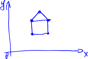
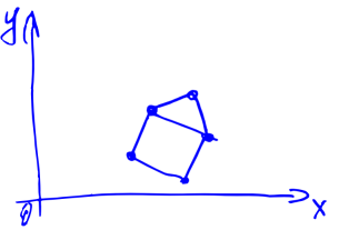
Suppose also that we are looking at the house from the origin in the direction of the OX. Now we turned a certain angle counterclockwise. Question: what will the house look like for us? Intuitively, the result will be approximately the same as in the image below.
But how to calculate the result? And, worst of all, how to do it in three-dimensional space? If, for example, we rotate the camera very tricky: first along the axis OZ, then OX, then OY?
')
The answers to these questions will give the article below. First, I will tell you how to represent a house in the form of numbers (that is, talk about vectors), then about what the angles between vectors are (that is, the scalar product) and finally, how to rotate the camera (about the rotation matrix).
Let's think about vectors. That is, the arrows with length and direction.
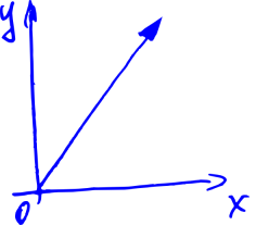
Attached to computer graphics — each such arrow sets a point in space.
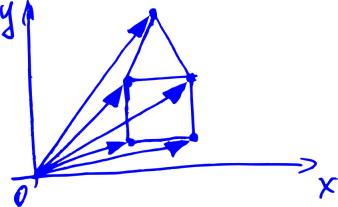
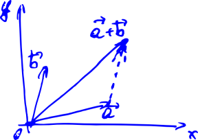
We want to learn how to rotate them. Because when we turn all the arrows in the picture above, we turn the house. Let's imagine that all we can do with these arrows is to add and multiply by a number. Like in school: to add two vectors, you need to draw a line from the beginning of the first vector to the end of the second.
For now we will focus on two-dimensional vectors. For a start, we would like to learn how to somehow write these vectors through numbers, because every time drawing them on paper in the form of arrows is not very convenient.
We will learn how to do this, remembering that any vector can be represented as the sum of some special vectors ( and Y), possibly multiplied by certain coefficients. These special vectors are called base vectors, and the coefficients are nothing more than the coordinates of our vector. If we denote basic vectors by (here i is the vector index, it is equal to either 1 or 2), the vector being considered is
  , and the coordinates of the latter as
  then we get the formula
(one)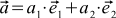
It can be shown that these coordinates will be unique for a given basis.
The benefits of the procedure of attributing coordinates to our arrows are obvious — before it was necessary to constantly draw an arrow to describe a vector, and now it is enough just to write two numbers — the coordinates of this vector. For example, we can agree to write like this: . Or so:
  . Then
  , but
, but  . Wonderful.
In real math, the procedure is somewhat different. First, we describe the properties that any objects must satisfy, so that we call them vectors. They are very natural. For example, vectors must support the operation of addition (two vectors) and multiplication by a number. The sum of two vectors should not depend on the order of the terms. The sum of the three vectors should not depend on the order in which we add them in pairs. And so on. The full list is on wikipedia .
If our all sorts of things satisfy these properties, then these things can be called vectors (this is such a duck typing). And the whole set of these pieces is a vector or linear space. The properties above are called axioms, and all the other properties of the vectors are derived from them (or linear space — hence the name “ linear algebra ”). For example, it can be inferred that among vectors there will be such special basis vectors through which any vector can be expressed using formula (1) and that this decomposition into coordinates will be unique for a given basis. Very quickly, it can be shown that our arrows just satisfy these axioms. The axiomatic approach is convenient, because if we encounter some other objects that satisfy the axioms, then we can immediately apply all the results of our theory to them. In addition, we avoid the definitions of arrows on the fingers at the beginning of the theory.
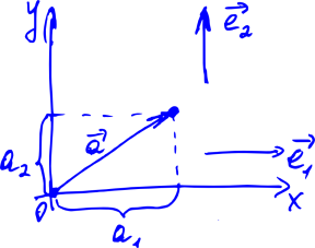
It can be easily shown (from those very axioms) that when adding vectors their corresponding coordinates will add up, and if the vector is multiplied by a number, all coordinates are multiplied by the same number. Now, to add two vectors, as in the picture below, we can not draw them (and not draw a line from the beginning of the first vector to the end of the second), but write, for example, .
.
Let's now introduce a special function of two arbitrary vectors a and b, which will be called the scalar product. We will refer to it like this: . These fashion brackets are scientifically called bra and ket vectors . There is no benefit from them yet, but it looks cool — moreover, this designation still has a deep meaning, especially if you go into mathematical details or quantum mechanics.
In the spirit of our axiomatic approach, we only require that the scalar product satisfy several axioms . If instead of the first vector we take the sum of the vectors of the type then we want to
  . Here Greek letters are factors, x and y are vectors. We also want that if we substitute such a sum for the second vector, we can do the same transformations (the scalar product of the sum of vectors also turns out to be the sum of scalar products, and the multipliers are also bracketed). In addition, we want the values
  always been non-negative. Finally, we want to equals zero if and only if the vector itself null. Oh, and also to
  .
.
If we add a ruler and a protractor to our arrows on paper, then these axioms will be satisfied by the function known from school: where the lengths of vectors are measured by a ruler, the angle between the vectors
  —Transporter.
If we do not have a ruler and protractor, then from the scalar product we can determine the length of the vector— —And the angle between vectors :
  . Of course, the angle depends on how the scalar product is defined.
Let's see how the scalar product is expressed through the individual coordinates of the vectors. Suppose we have two vectors a and b , which look like this: ,
,  . Then
  .
.
It does not look very much. To make life better, we will continue to work only with special coordinate systems. We will choose only those coordinate systems in which the basis vectors are of unit length and perpendicular to each other. In other words,
(2a) , if a
(2b) , if a
Such vectors are called orthonormal. The expression for the scalar product in orthonormal coordinate systems is transformed beyond recognition:
(3)
All coordinate systems in this article are assumed to be orthonormal. Surprisingly, it follows from our construction that the result of formula (3) does not depend on which orthonormal basis for coordinates is chosen.
Carefully looking at the picture “Decomposition of a vector into coordinates” (it is shown again after this paragraph), one may suspect that the coordinate of the vector is nothing more than its projection onto the corresponding base vector. That is, the scalar product of the original vector with one of the basis vectors:
(four)
Indeed, for example, . It seems that this is a tautology, because the coordinates of the basis vectors in their own basis will always be (1, 0) and (0, 1). But we can take other basic vectors, and express them through the old basis. For example, a new orthonormal basis may look in the old basis as
  and
and  . And then we can determine, for example, the first coordinate of the vector in the new basis by the formula (4) as
  .
.
The meticulous reader will say, “but you see, formula (3) can be used as a scalar product definition, and then we don’t need any orthonormal base vectors”. And it will be right that formula (3) can work as one of the definitions of the scalar product. But there is a subtle point: then we need to show that when the coordinate system is changed, the same formula, but with the coordinates of vectors a and b from another basis, will give the same number. And this will be only if all bases are orthonormal. This can be shown by reading the following section.
Let's find out how the coordinates of vectors change, if we change the whole coordinate system. Why do we need to change the coordinate system at all? If you think a little, it becomes clear that the rotation of the coordinate system is equivalent to turning the camera in 3D or 2D modeling (see below a slightly modified drawing with a house). So learning how to rotate the coordinate system is just what we need.
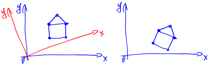
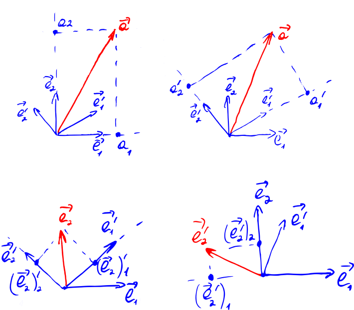
Let's denote the i-th coordinate of the vector a in the new coordinate system as , and new basis vectors as
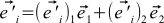
  . In addition, we denote the jth coordinate of the OLD basis vector i in the NEW basis as
  . Finally, we denote the i-th coordinate of the NEW basis vector j in the OLD basis as
  . Now we can express the source vector and the old basis vectors in terms of the new basis vectors. Namely
(five)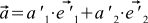 and
and
(6)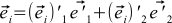
In addition, you can express the new basis vectors through the old:
(7)
Some of these expansions are shown in the image below.
Now we simply rewrite the formula (1) through the vectors of the new base:
If we compare this with formula (5), and recall that the coordinates of the vectors are uniquely determined, we can see that
(eight) and
and 
It's amazing how these formulas look like equations (3)! They look like the dot product of a vector. with certain vectors (below we show that this is not an accident).
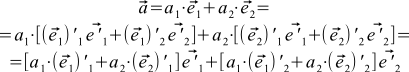
If we write equations (9) with one formula, we get
(9)
This formula can be derived differently by combining (4), (1) and (7): . If we recall the properties of the inner product, then this formula splits into four sums. Now, if we recall that our basic vectors are orthonormal, we get
  .
.
This formula does not look exactly like formula (9): instead of stand here
  . This is not a mistake — just
  . That is, the j -th coordinate of the OLD basis vector i in the NEW basis
  always equal to the i -th coordinate of the NEW basis vector j in the OLD basis,
  . This will become obvious if you try to express these coordinates through the formula (4):
(ten) ,
, 
And the scalar product, as we remember, does not depend on the order of the product of vectors.
This will become even more obvious if we recall that these scalar products are the angles between different (unit) basis vectors. These angles, of course, do not depend on whether to postpone them counterclockwise or counterclockwise.
If you are familiar with matrices, then formula (9) (two formulas) can be rewritten in matrix form.
(eleven)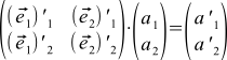
What does this all mean? As usual, there is no magic here — we just agree that multiplying this number plate from the left by the vector on the right is calculated as formula (9). That is, we multiply each line of the plate by a column to the right (as if we are doing the scalar product of two vectors), and write the results one after the other, also getting a column.
It is possible, by the way, to extend this rule to the multiplication of two plates: let's agree to multiply each line of the first plate on each second column, and write the results on the plate too: we will write down the first line multiply with the third column in the first line and the third column. Formula (11) then becomes a particular case of this rule. Schematically, this is all shown in the figure below.
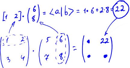
The plates from numbers supplied with such a rule of multiplication by vectors and other plates will be called matrices.
The rule of matrix multiplication looks even more natural if we find out that the scalar product, as we agreed to denote it, , on the most it assumes that vector a is a string, and vector b is a column. Before that, we agreed to write vectors in columns, and the row vector a actually is not just an inverted vector a , but an object of a special dual vector space . But in the case of orthonormal bases, the coordinates of the original and dual vectors are the same (that is, the a-row and a-column are the same), so these details do not affect our presentation. It's okay In addition, on the other hand, the formula (3) for the scalar product is a special case of matrix multiplication.
In general, it can be shown that multiplication by matrices corresponds to certain transformations of vectors. Instead of "transformation" it is customary to say operators . And multiplication by a matrix is a linear operator. In addition, for any linear operator there is one and only one matrix of the operator. About what it is, you can read on Wikipedia . If you describe it here, the article will never end.
So, as we found out, turning the coordinate system is equivalent to turning the camera in 3D or 2D modeling. Therefore, the matrix from formula (11) is called the rotation matrix. Formula (11) can be interpreted not as a replacement for the coordinate system, but as a description of the rotation operator.
It is not entirely clear how to calculate this matrix. It is easy if we turn to formulas (10) and recall that the cosine of the angle between unit vectors is equal to their scalar product. Then, for example,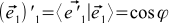 where
where  —An angle of rotation of the coordinate system (camera). It is, by definition, positive if the rotation is counterclockwise, and negative when it is rotated clockwise (see the picture just below — it was already, but now it is relevant again). If you tinker a bit with geometry or trigonometry, you can find out that the entire rotation matrix looks like this:
(12a)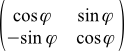
If you look at Wikipedia , the formula there looks a little different:
(12b)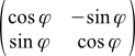
This is all because in it is the angle of rotation of the vectors themselves (or of our house type objects). It is also considered positive if the rotation is counterclockwise. But the rotation of the camera is opposite to the rotation of objects, that is, the angle of rotation of the camera is equal to the angle of rotation of objects, but taken with the opposite sign.
Again actual drawing:
These matrices are very convenient things. They can be multiplied and put together, not only two, but three and four each. Matrices can be denoted by capital letters. For example, T is the usual designation for rotation matrices (it certainly depends on how the system or camera is rotated). Then formula (11) goes to .
.
Matrices have a unit matrix — in the sense that any vector, being multiplied by it to the left, remains itself. And any matrix, too. The unit matrix looks like a table, all filled with zeros, only units on the diagonal. Such a matrix corresponds to a rotation of zero degrees. That is, the absence of a turn. She looks like this:
(13)
If you count or think a little, the multiplication of the rotation matrices corresponds to several turns, performed one after the other (but in a different order — from right to left). So if in your program there are several predetermined turns in a row, then do not rush to use them for all points in your three-dimensional world. It is better to multiply the matrix, get a common rotation matrix, and already apply it.
For many matrices, it is possible to find such that when multiplying the first by the second, the unit matrix is obtained. These new matrices are called inverse, and for T they are denoted as . I.e
. I.e 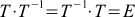 .
.
If you think a little more, then such a matrix must correspond to the opposite for T turn — one that neutralizes T. This is very convenient. If you learn to calculate the inverse matrix, you can easily rotate the camera back, if necessary.
If you think quite a bit, and even count a little, then for the rotation matrices, due to the fact that they have a special structure (see formula (10)), it is very easy to get inverse matrices: it is enough just to rotate the matrix along the diagonal from the upper left in the lower right corner (of the diagonal itself, along which there are units in the unit matrix). This operation is called transposition . It is much (much, much) faster than the search for the inverse matrix in the general case.
Finally, we turn to three-dimensional space. All formulas are transformed trivially — there are three coordinates in the vectors, three sums in the scalar product, and so on.
The difficulty arises only with the rotation matrix. Intuitively, it is almost obvious that we can represent any turn in the form of a sequence of three turns (along OX, OY, OZ) (however, we must work a bit to show it) —so that any rotation can be specified with these three turning angles. Three matrices corresponding to these rotations can be multiplied, and a common matrix can be obtained for any three-dimensional rotation (with three parameters — angle of rotation relative to the coordinate axes). Her view can be found on wikipedia .
It can be shown that instead of three corners, any three-dimensional rotation can be defined by a vector around which rotation takes place and by an angle to which we rotate the camera along this vector (we will set it counterclockwise, when viewed from the end of the vector). Oddly enough (or rather, of course), this method also requires three numbers. Since the length of the vector is not important to us, we can make it a unit length. Then, in order to set it, we need only two numbers (for example, two angles — say, relative to OX and OY). An angle is added to these two numbers, which we will rotate relative to the vector. The formula for the rotation matrix with these parameters can also be found on Wikipedia .
That's all, thank you for your attention.
PS In the process of preparing the article, it turned out that the formulas look a bit blurry, although they seem to have been saved from 600 dpi to png. Apparently, so badly Inkscape saves small pngs. I wildly apologize for this, but I have no strength to rework.
PPS Although the pictures are uploaded to habrastorage, but sometimes some are not displayed. Apparently, some problems with habrastorage. Try simply reload the page.
Introduction
Task. Suppose that we have a two-dimensional picture, as below (house).
Suppose also that we are looking at the house from the origin in the direction of the OX. Now we turned a certain angle counterclockwise. Question: what will the house look like for us? Intuitively, the result will be approximately the same as in the image below.
But how to calculate the result? And, worst of all, how to do it in three-dimensional space? If, for example, we rotate the camera very tricky: first along the axis OZ, then OX, then OY?
')
The answers to these questions will give the article below. First, I will tell you how to represent a house in the form of numbers (that is, talk about vectors), then about what the angles between vectors are (that is, the scalar product) and finally, how to rotate the camera (about the rotation matrix).
Vector coordinates
Let's think about vectors. That is, the arrows with length and direction.
Attached to computer graphics — each such arrow sets a point in space.
We want to learn how to rotate them. Because when we turn all the arrows in the picture above, we turn the house. Let's imagine that all we can do with these arrows is to add and multiply by a number. Like in school: to add two vectors, you need to draw a line from the beginning of the first vector to the end of the second.
For now we will focus on two-dimensional vectors. For a start, we would like to learn how to somehow write these vectors through numbers, because every time drawing them on paper in the form of arrows is not very convenient.
We will learn how to do this, remembering that any vector can be represented as the sum of some special vectors ( and Y), possibly multiplied by certain coefficients. These special vectors are called base vectors, and the coefficients are nothing more than the coordinates of our vector. If we denote basic vectors by
(here i is the vector index, it is equal to either 1 or 2), the vector being considered is , and the coordinates of the latter as then we get the formula(one)
It can be shown that these coordinates will be unique for a given basis.
The benefits of the procedure of attributing coordinates to our arrows are obvious — before it was necessary to constantly draw an arrow to describe a vector, and now it is enough just to write two numbers — the coordinates of this vector. For example, we can agree to write like this:
. Or so: . Then , but . Wonderful.In real math, the procedure is somewhat different. First, we describe the properties that any objects must satisfy, so that we call them vectors. They are very natural. For example, vectors must support the operation of addition (two vectors) and multiplication by a number. The sum of two vectors should not depend on the order of the terms. The sum of the three vectors should not depend on the order in which we add them in pairs. And so on. The full list is on wikipedia .
If our all sorts of things satisfy these properties, then these things can be called vectors (this is such a duck typing). And the whole set of these pieces is a vector or linear space. The properties above are called axioms, and all the other properties of the vectors are derived from them (or linear space — hence the name “ linear algebra ”). For example, it can be inferred that among vectors there will be such special basis vectors through which any vector can be expressed using formula (1) and that this decomposition into coordinates will be unique for a given basis. Very quickly, it can be shown that our arrows just satisfy these axioms. The axiomatic approach is convenient, because if we encounter some other objects that satisfy the axioms, then we can immediately apply all the results of our theory to them. In addition, we avoid the definitions of arrows on the fingers at the beginning of the theory.
It can be easily shown (from those very axioms) that when adding vectors their corresponding coordinates will add up, and if the vector is multiplied by a number, all coordinates are multiplied by the same number. Now, to add two vectors, as in the picture below, we can not draw them (and not draw a line from the beginning of the first vector to the end of the second), but write, for example,
.Scalar product
Let's now introduce a special function of two arbitrary vectors a and b, which will be called the scalar product. We will refer to it like this:
. These fashion brackets are scientifically called bra and ket vectors . There is no benefit from them yet, but it looks cool — moreover, this designation still has a deep meaning, especially if you go into mathematical details or quantum mechanics.In the spirit of our axiomatic approach, we only require that the scalar product satisfy several axioms . If instead of the first vector we take the sum of the vectors of the type
then we want to . Here Greek letters are factors, x and y are vectors. We also want that if we substitute such a sum for the second vector, we can do the same transformations (the scalar product of the sum of vectors also turns out to be the sum of scalar products, and the multipliers are also bracketed). In addition, we want the values always been non-negative. Finally, we want to equals zero if and only if the vector itself null. Oh, and also to .If we add a ruler and a protractor to our arrows on paper, then these axioms will be satisfied by the function known from school:
where the lengths of vectors are measured by a ruler, the angle between the vectors —Transporter.If we do not have a ruler and protractor, then from the scalar product we can determine the length of the vector—
—And the angle between vectors : . Of course, the angle depends on how the scalar product is defined.Let's see how the scalar product is expressed through the individual coordinates of the vectors. Suppose we have two vectors a and b , which look like this:
, . Then .It does not look very much. To make life better, we will continue to work only with special coordinate systems. We will choose only those coordinate systems in which the basis vectors are of unit length and perpendicular to each other. In other words,
(2a)
, if a (2b)
, if a Such vectors are called orthonormal. The expression for the scalar product in orthonormal coordinate systems is transformed beyond recognition:
(3)
All coordinate systems in this article are assumed to be orthonormal. Surprisingly, it follows from our construction that the result of formula (3) does not depend on which orthonormal basis for coordinates is chosen.
Carefully looking at the picture “Decomposition of a vector into coordinates” (it is shown again after this paragraph), one may suspect that the coordinate of the vector is nothing more than its projection onto the corresponding base vector. That is, the scalar product of the original vector with one of the basis vectors:
(four)
Indeed, for example,
. It seems that this is a tautology, because the coordinates of the basis vectors in their own basis will always be (1, 0) and (0, 1). But we can take other basic vectors, and express them through the old basis. For example, a new orthonormal basis may look in the old basis as and . And then we can determine, for example, the first coordinate of the vector in the new basis by the formula (4) as .The meticulous reader will say, “but you see, formula (3) can be used as a scalar product definition, and then we don’t need any orthonormal base vectors”. And it will be right that formula (3) can work as one of the definitions of the scalar product. But there is a subtle point: then we need to show that when the coordinate system is changed, the same formula, but with the coordinates of vectors a and b from another basis, will give the same number. And this will be only if all bases are orthonormal. This can be shown by reading the following section.
Rotate Coordinate System
Let's find out how the coordinates of vectors change, if we change the whole coordinate system. Why do we need to change the coordinate system at all? If you think a little, it becomes clear that the rotation of the coordinate system is equivalent to turning the camera in 3D or 2D modeling (see below a slightly modified drawing with a house). So learning how to rotate the coordinate system is just what we need.
Let's denote the i-th coordinate of the vector a in the new coordinate system as
, and new basis vectors as . In addition, we denote the jth coordinate of the OLD basis vector i in the NEW basis as . Finally, we denote the i-th coordinate of the NEW basis vector j in the OLD basis as . Now we can express the source vector and the old basis vectors in terms of the new basis vectors. Namely(five)
and(6)
In addition, you can express the new basis vectors through the old:
(7)
Some of these expansions are shown in the image below.
Now we simply rewrite the formula (1) through the vectors of the new base:
If we compare this with formula (5), and recall that the coordinates of the vectors are uniquely determined, we can see that
(eight)
and It's amazing how these formulas look like equations (3)! They look like the dot product of a vector.
with certain vectors (below we show that this is not an accident).If we write equations (9) with one formula, we get
(9)
This formula can be derived differently by combining (4), (1) and (7):
. If we recall the properties of the inner product, then this formula splits into four sums. Now, if we recall that our basic vectors are orthonormal, we get .This formula does not look exactly like formula (9): instead of
stand here . This is not a mistake — just . That is, the j -th coordinate of the OLD basis vector i in the NEW basis always equal to the i -th coordinate of the NEW basis vector j in the OLD basis, . This will become obvious if you try to express these coordinates through the formula (4):(ten)
, And the scalar product, as we remember, does not depend on the order of the product of vectors.
This will become even more obvious if we recall that these scalar products are the angles between different (unit) basis vectors. These angles, of course, do not depend on whether to postpone them counterclockwise or counterclockwise.
Rotation matrix
If you are familiar with matrices, then formula (9) (two formulas) can be rewritten in matrix form.
(eleven)
What does this all mean? As usual, there is no magic here — we just agree that multiplying this number plate from the left by the vector on the right is calculated as formula (9). That is, we multiply each line of the plate by a column to the right (as if we are doing the scalar product of two vectors), and write the results one after the other, also getting a column.
It is possible, by the way, to extend this rule to the multiplication of two plates: let's agree to multiply each line of the first plate on each second column, and write the results on the plate too: we will write down the first line multiply with the third column in the first line and the third column. Formula (11) then becomes a particular case of this rule. Schematically, this is all shown in the figure below.
The plates from numbers supplied with such a rule of multiplication by vectors and other plates will be called matrices.
The rule of matrix multiplication looks even more natural if we find out that the scalar product, as we agreed to denote it,
, on the most it assumes that vector a is a string, and vector b is a column. Before that, we agreed to write vectors in columns, and the row vector a actually is not just an inverted vector a , but an object of a special dual vector space . But in the case of orthonormal bases, the coordinates of the original and dual vectors are the same (that is, the a-row and a-column are the same), so these details do not affect our presentation. It's okay In addition, on the other hand, the formula (3) for the scalar product is a special case of matrix multiplication.In general, it can be shown that multiplication by matrices corresponds to certain transformations of vectors. Instead of "transformation" it is customary to say operators . And multiplication by a matrix is a linear operator. In addition, for any linear operator there is one and only one matrix of the operator. About what it is, you can read on Wikipedia . If you describe it here, the article will never end.
So, as we found out, turning the coordinate system is equivalent to turning the camera in 3D or 2D modeling. Therefore, the matrix from formula (11) is called the rotation matrix. Formula (11) can be interpreted not as a replacement for the coordinate system, but as a description of the rotation operator.
It is not entirely clear how to calculate this matrix. It is easy if we turn to formulas (10) and recall that the cosine of the angle between unit vectors is equal to their scalar product. Then, for example,
where —An angle of rotation of the coordinate system (camera). It is, by definition, positive if the rotation is counterclockwise, and negative when it is rotated clockwise (see the picture just below — it was already, but now it is relevant again). If you tinker a bit with geometry or trigonometry, you can find out that the entire rotation matrix looks like this:(12a)
If you look at Wikipedia , the formula there looks a little different:
(12b)
This is all because
in it is the angle of rotation of the vectors themselves (or of our house type objects). It is also considered positive if the rotation is counterclockwise. But the rotation of the camera is opposite to the rotation of objects, that is, the angle of rotation of the camera is equal to the angle of rotation of objects, but taken with the opposite sign.Again actual drawing:
Pleasant trifles
These matrices are very convenient things. They can be multiplied and put together, not only two, but three and four each. Matrices can be denoted by capital letters. For example, T is the usual designation for rotation matrices (it certainly depends on how the system or camera is rotated). Then formula (11) goes to
.Matrices have a unit matrix — in the sense that any vector, being multiplied by it to the left, remains itself. And any matrix, too. The unit matrix looks like a table, all filled with zeros, only units on the diagonal. Such a matrix corresponds to a rotation of zero degrees. That is, the absence of a turn. She looks like this:
(13)
If you count or think a little, the multiplication of the rotation matrices corresponds to several turns, performed one after the other (but in a different order — from right to left). So if in your program there are several predetermined turns in a row, then do not rush to use them for all points in your three-dimensional world. It is better to multiply the matrix, get a common rotation matrix, and already apply it.
For many matrices, it is possible to find such that when multiplying the first by the second, the unit matrix is obtained. These new matrices are called inverse, and for T they are denoted as
. I.e .If you think a little more, then such a matrix
must correspond to the opposite for T turn — one that neutralizes T. This is very convenient. If you learn to calculate the inverse matrix, you can easily rotate the camera back, if necessary.If you think quite a bit, and even count a little, then for the rotation matrices, due to the fact that they have a special structure (see formula (10)), it is very easy to get inverse matrices: it is enough just to rotate the matrix along the diagonal from the upper left in the lower right corner (of the diagonal itself, along which there are units in the unit matrix). This operation is called transposition . It is much (much, much) faster than the search for the inverse matrix in the general case.
Three-dimensional space
Finally, we turn to three-dimensional space. All formulas are transformed trivially — there are three coordinates in the vectors, three sums in the scalar product, and so on.
The difficulty arises only with the rotation matrix. Intuitively, it is almost obvious that we can represent any turn in the form of a sequence of three turns (along OX, OY, OZ) (however, we must work a bit to show it) —so that any rotation can be specified with these three turning angles. Three matrices corresponding to these rotations can be multiplied, and a common matrix can be obtained for any three-dimensional rotation (with three parameters — angle of rotation relative to the coordinate axes). Her view can be found on wikipedia .
It can be shown that instead of three corners, any three-dimensional rotation can be defined by a vector around which rotation takes place and by an angle to which we rotate the camera along this vector (we will set it counterclockwise, when viewed from the end of the vector). Oddly enough (or rather, of course), this method also requires three numbers. Since the length of the vector is not important to us, we can make it a unit length. Then, in order to set it, we need only two numbers (for example, two angles — say, relative to OX and OY). An angle is added to these two numbers, which we will rotate relative to the vector. The formula for the rotation matrix with these parameters can also be found on Wikipedia .
That's all, thank you for your attention.
PS In the process of preparing the article, it turned out that the formulas look a bit blurry, although they seem to have been saved from 600 dpi to png. Apparently, so badly Inkscape saves small pngs. I wildly apologize for this, but I have no strength to rework.
PPS Although the pictures are uploaded to habrastorage, but sometimes some are not displayed. Apparently, some problems with habrastorage. Try simply reload the page.
Source: https://habr.com/ru/post/234203/
All Articles