About the Bayes Formula, Predictions and Confidence Intervals
Habré has many articles on this topic, but they do not consider practical problems. I will try to correct this unfortunate misunderstanding. Bayes Formula is used for spam filtering, recommendation services and ratings. Without it, a significant number of fuzzy search algorithms would be impossible. In addition, this formula was the cause of holivar among mathematicians.
Let's start from afar. If the occurrence of one event increases or decreases the likelihood of another, then such events are called dependent. Turver does not study cause and effect relationships. Therefore, dependent events are not necessarily the consequences of each other, the connection may not be obvious. For example, “a person has blue eyes” and “a person knows Arabic” are dependent events, since Arabs have blue eyes very rarely.
')
Now you should enter the notation.
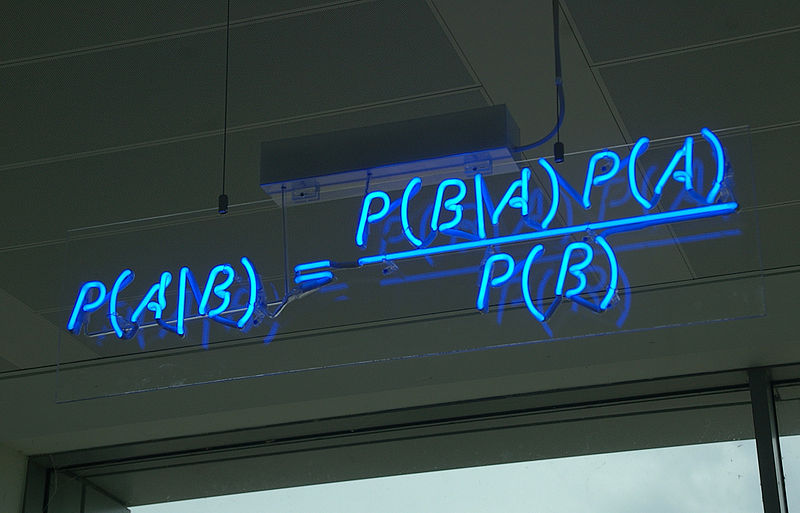
Let's think what is the probability of the occurrence of two events at the same time. P (AB). The probability of the first event multiplied by the probability of the second event, in the case of the first. P (AB) = P (A) P (B | A). Now, if we recall that P (AB) = P (BA). We obtain P (A) P (B | A) = P (B) P (A | B). Move P (B) to the left and get the Bayes formula:
Everything is so simple that 300 years ago a simple priest derived this formula. But this does not diminish the practical value of this theorem. It allows you to solve the "reverse problem": according to test data, assess the situation.
The direct problem can be described as follows: for the reason to find the probability of one of the consequences. For example, an absolutely symmetrical coin is given (the probability of falling of an eagle, as well as tails, is 1/2). It is necessary to calculate the probability that if we throw a coin twice, an eagle will fall both times. Obviously, it is equal to 1/2 * 1/2 = 1/4.
But the problem is that we know the probability of an event only in a minority of cases, almost all of which are artificial, for example, gambling. At the same time, there is nothing absolute in nature, the probability of a falling of an eagle in a real coin is 1/2 only approximately. It can be said that the direct problem studies some spherical horses in a vacuum.
In practice, the inverse problem is more important: to evaluate the situation according to test data. But the problem of the inverse problem is that its solution is more difficult. Mainly due to the fact that our solution is not a point P = C, but some function P = f (x).
For example, we have a coin, we need to evaluate with the help of experiments the probability of tails falling out. If we threw a coin 1 time and an eagle fell, this does not mean that eagles always fall out. If you threw it 2 times and got 2 eagles, then again this does not mean that only eagles fall out. To get exactly the probability of a tail, we must throw a coin an infinite number of times. In practice, this is not possible and we always calculate the probability of an event with some accuracy.
We have to use some function. Usually it is usually denoted as P (p = x | s lattices, f eagles) and called the probability density. It reads like a probability, that the probability of falling of an eagle is equal to x, if according to the experimental data s tails and f eagles were dropped. It sounds difficult because of taftology. It is easier to consider p as a certain property of the coin, and not as a probability. And read: so the probability that p = x ...
Looking ahead, I’ll say that if we throw 1000 times into the first coin and get 500 eagles, and get the second 10,000 and get 5000 eagles, then the probability densities will look like this:

Due to the fact that we do not have a point, but a curve, we are forced to use confidence intervals. For example, if they say 80% confidence interval for p is 45% to 55%, then this means that with 80% probability p lies between 45% and 55%.
For simplicity, we will consider the binomial distribution. This is the distribution of the number of “successes” in a sequence of a number of independent random experiments, such that the probability of “success” in each of them is constant. It is observed almost always when we have a test sequence with two possible outcomes. For example, when we throw a coin a few times, or evaluate the banner CTR, or conversion on the site.
For example, we assume that we need to estimate the probability of a tails coin. We threw a coin a number of times and got f eagles and s tails. Denote this event as [s, f] and substitute it in the Bayes formula instead of B. The event when p is equal to some number will be denoted as p = x and substitute instead of event A.
P ([s, d] | p = x); Probability to get [s, d] if p = x, provided that p = x we know P ([s, f] | p = x) = K ( f, s) * x ^ s (1-x) ^ f. Where K (f, s) is the binomial coefficient. We get:

We do not know P ([s, f]). Yes, and the binomial coefficient is problematic to calculate: there factorials. But these problems can be solved: the total probability of all possible x must be equal to 1.
Using simple transformations, we get the formula:
It is programmed simply, just 10 lines:
However, we still have P (p = x) unknown. It expresses how likely it is that p = x, if we have no experimental data. This function is called a priori. Because of it, holivar occurred in probability theory. We cannot calculate a priori strictly mathematically, just to ask subjectively. And without a priori we cannot solve the inverse problem.
Proponents of the classical interpretation (frequency approach, PE), believe that all possible p are equally probable before the experiment. Those. before the experiment, it is necessary to “forget” those data that are known to us before it. Their opponents, supporters of the Bayesian approach (BP), believe that it is necessary to ask some a priori on the basis of our knowledge before the start of the experiment. These are fundamental differences, even the definition of the concept of probability is different for these groups.
By the way, the creator of this formula, Thomas Baise, died 200 years earlier than holivar, and only indirectly related to this dispute. Bayes Formula is part of both competing theories.
Frequency approach (PE) is better suited for science, where you need to objectively prove some kind of hypothesis. For example, the fact that the death rate from the drug is less than a certain threshold. If you need, taking into account all available information, to make a decision, it is better to use the PSU.
PE is not suitable for prediction. By the way, the formula of the confidence intervals, consider the confidence interval for the state of emergency. Proponents of BP usually use Beta distribution as a priori for the binomial distribution, with a = 1 and b = 1 it degenerates into a continuous distribution that their opponents use. As a result, the formula takes the form:
=x^{s+\alpha%20-1}%20(1-x)^{f+\beta%20-1}%20\\P(p=x|[s,f])=\frac{T(x)}{\int_{0}^{1}{%20T(t)dt}})
This is a universal formula. When using a PE, b = a = 1 must be specified. Proponents of BP should in some way choose these parameters so that a plausible beta distribution is obtained. Knowing a and b, you can use the formulas of PE, for example, to calculate the confidence interval. For example, we chose a = 4.5, b = 20, we have 50 successes and 100 failures; in order to calculate the confidence interval in the PD, we need to enter 53.5 (50 + 4.5-1) success and 119 failure into the usual formula.
However, we have no criteria for choosing a and b. The next chapter will tell you how to select them by static data.
Most logical as a forecast to use the mat. expectation. Its formula is easily obtained from the formula mat. Beta expectations. We get:
 .
.
For example, we have a website with articles. Each of them has a "like" button. If we sort by the number of likes, then new articles have little chance to kill old ones. If we sort by the ratio of likes to visits, articles with one entry and one like will interrupt an article with 1000 visits and with 999 likes. It is more reasonable to sort by the last formula, but you need to somehow define a and b. The easiest way through the 2 main points of the beta distribution: mat. expectation (how much will be on average) and variance (what is the average deviation from the average).
Let L be the average probability of a like. From the expectation of the beta distribution L = a / (a + b) => a + b = a / L => aL + bL = a => b = a (1 / L - 1). Substitute in the dispersion formula:
^2(a+b+1)}=\frac{a^2(1/L%20-%201)}{(a/L)^2(a/L+1)}=\frac{1/L%20-%201}{(1/L)^2(a/L+1)}%20\\(a/L+1)D=\frac{1/L%20-%201}{(1/L)^2}%20\\a=\frac{1%20-%20L}{(1/L)^2D}-L)
On pseudocode, it will look like this:
Despite the fact that this choice of a and b seems to be objective. This is not strict mathematics. First of all, it’s not a fact that article likeability is subject to Beta distribution, in contrast to the binomial distribution, this distribution is not “physical”; it is introduced for convenience. We essentially adjusted the curve to the statistics. Moreover, there are several options for fitting.
For example, we conducted an A / B test of several site design options. Got some results and think about whether to stop it. If we stop too early, we can choose the wrong option, but we still need to stop once. We can estimate confidence intervals, but their analysis is difficult. At a minimum, because depending on the coefficient of significance, we have different confidence intervals. Now I will show you how to calculate the probability that one option is better than all the others.
In addition to dependent events, there are independent events. For such events, P (A | B) = P (A). Therefore, P (AB) = P (B) P (A | B) = P (A) P (B). First you need to show that the options are independent. By the way, to compare the confidence intervals correctly, only in the case when the options are independent. As already mentioned, supporters of PE drop all data except the experiment itself. Variants are separate experiments, so each of them depends only on its results. Therefore, they are independent.
For BP, the proof is more complicated, the main point that a priori “isolates” the variants from each other. For example, the events “blue eyes” and “knows Arabic” are dependent, and the events “Arab knows Arabic” and “Arabic has blue eyes” do not exist, since the relationship between the first two events is exhausted by the event “Arab man”. A more correct record of P (p = x) in our case is the following: P (p = x | apriori = f (x)). Since everything depends on the choice of function a priori. And the events P (p i = x | apriori = f (x)) and P (p j = x | apriori = f (x)) are independent, since the only relationship between them is a function a priori.
We introduce the definition of P (p <x), the probability that p is less than x. The formula is obvious:
}=\int_{0}^{x}{P(p=t|[s,f])}%20dt)
We simply “added” all point probabilities.
Now let's digress, and I will explain to you the formula for total probability. Suppose there are 3 events A, B, W. The first two events are mutually exclusive and one of them must occur. Those. Of these two events, no more and no less than one always occur. Those. either one or the other should happen, but not together. This is for example the gender of a person or the falling of an eagle / tail in one throw. So, the Event W can occur only in 2 cases: together with A and together with B. P (W) = P (AW) + P (BW) = P (A) * P (W | A) + P (B) * P (W | B). Similarly, it happens when there are more events. Even when their number is infinite. Therefore, we can make such transformations:
=\int_{0}^{1}{P(p=x)P(W|p=x)dx})
Suppose we have n options. We know for each of the number of successes and failures. [s_1, f_1], ..., [s_n, f_n]. To simplify the recording, we will miss the data from the recording. Those. instead of P (W | [s_1, f_1], ..., [s_n, f_n]) we simply write: P (W). Let us denote the probability that option i is better than all the others (Chance To Beat All) and make some reduction in the record:
=P(best=i))
∀j ≠ i means for any j not equal to i. In simple terms, this all means the probability that p i is the most.
Let us apply the formula of total probability:
%20=\int_{0}^{1}{P(p_i=x)P(best=i|p_i=x)}dx)
%20=\\=P(p_i%3Ep_j,%20\forall%20j\neq%20i%20|p_i=x)%20=\\=P(p_j%3Cx,%20\forall%20j\neq%20i%20|p_i=x)%20=\\=P(p_j%3Cx,%20\forall%20j\neq%20i)%20=\\=\prod_{j\neq%20i}^{{}}{P(p_j%3Cx)})
The first conversion simply changes the form of the record. The second substitutes x instead of p i , since we have a conditional probability. Since p_i is independent of p_j, a third transformation can be performed. As a result, we obtained that this is equal to the probability that all p_j except i are less than x. Since the options are independent, then P (AB) = P (A) * P (B) holds. Those. this is all transformed into a product of probabilities.
As a result, the formula will look like:
=\int_{0}^{1}{P(p_i=x)\prod_{j\neq%20i}^{{}}{P(p_j%3Cx)}}dx)
This can all be calculated in linear time:
For a simple case when there are only two options (Chance to beat baseline / origin, CTBO). using a normal approximation, we can calculate this chance in constant time . In general, it is impossible to solve in constant time. At least, Google did not succeed in Google WebSite Optimizer and had CTBA and CTBO, after transferring to Analytics, CTBO remained less convenient. The only explanation for this is that there is too much resources spent on calculating CTBA.
By the way, you can understand if you organized the algorithm correctly by two things. Total CTBA should be equal to 1. You can also compare your result with screenshots of Google WebSite Optimizer. Here is a comparison of the results of our free statistical calculator HTraffic Calc with Google WebSite Optimizer.

The difference in the last comparison is due to the fact that I use “smart rounding”. Without rounding, the data is the same.
In general, you can HTraffic Calc to test your code, because unlike Google WebSite Optimizer, it allows you to enter your data. You can also compare options with it, however, you should consider the fundamental features of CTBA.
If the success rate is far from 0.5. At the same time, the number of tests (for example, coin flips or banner impressions) is small in some variants and the number of tests differs several times in several variants, then you must either set Apriori or equalize the number of tests. The same applies not only to the CTBA, but also to the comparison of confidence intervals.

As we see from the screenshot of the second option, the chances are higher to beat the first one. This is due to the fact that we selected a uniform distribution as a priori, and his expectation mat is 0.5, this is more than 0.3, so in this case the variant with a smaller number of tests received some bonus. From the point of view of PE, the experiment is broken - all variants should have an equal number of tests. You must equalize the number of tests, discarding part of the tests from one of the options. Or use the power supply and choose a priori.
Introduction
Let's start from afar. If the occurrence of one event increases or decreases the likelihood of another, then such events are called dependent. Turver does not study cause and effect relationships. Therefore, dependent events are not necessarily the consequences of each other, the connection may not be obvious. For example, “a person has blue eyes” and “a person knows Arabic” are dependent events, since Arabs have blue eyes very rarely.
')
Now you should enter the notation.
- P (A) means the probability of an event A.
- P (AB) probability of both events occurring together. It does not matter in what order the events occur P (AB) = P (BA).
- P (A | B) probability of the occurrence of event A, if event B occurred.
Let's think what is the probability of the occurrence of two events at the same time. P (AB). The probability of the first event multiplied by the probability of the second event, in the case of the first. P (AB) = P (A) P (B | A). Now, if we recall that P (AB) = P (BA). We obtain P (A) P (B | A) = P (B) P (A | B). Move P (B) to the left and get the Bayes formula:
Everything is so simple that 300 years ago a simple priest derived this formula. But this does not diminish the practical value of this theorem. It allows you to solve the "reverse problem": according to test data, assess the situation.
Direct and inverse problems
The direct problem can be described as follows: for the reason to find the probability of one of the consequences. For example, an absolutely symmetrical coin is given (the probability of falling of an eagle, as well as tails, is 1/2). It is necessary to calculate the probability that if we throw a coin twice, an eagle will fall both times. Obviously, it is equal to 1/2 * 1/2 = 1/4.
But the problem is that we know the probability of an event only in a minority of cases, almost all of which are artificial, for example, gambling. At the same time, there is nothing absolute in nature, the probability of a falling of an eagle in a real coin is 1/2 only approximately. It can be said that the direct problem studies some spherical horses in a vacuum.
In practice, the inverse problem is more important: to evaluate the situation according to test data. But the problem of the inverse problem is that its solution is more difficult. Mainly due to the fact that our solution is not a point P = C, but some function P = f (x).
For example, we have a coin, we need to evaluate with the help of experiments the probability of tails falling out. If we threw a coin 1 time and an eagle fell, this does not mean that eagles always fall out. If you threw it 2 times and got 2 eagles, then again this does not mean that only eagles fall out. To get exactly the probability of a tail, we must throw a coin an infinite number of times. In practice, this is not possible and we always calculate the probability of an event with some accuracy.
We have to use some function. Usually it is usually denoted as P (p = x | s lattices, f eagles) and called the probability density. It reads like a probability, that the probability of falling of an eagle is equal to x, if according to the experimental data s tails and f eagles were dropped. It sounds difficult because of taftology. It is easier to consider p as a certain property of the coin, and not as a probability. And read: so the probability that p = x ...
Looking ahead, I’ll say that if we throw 1000 times into the first coin and get 500 eagles, and get the second 10,000 and get 5000 eagles, then the probability densities will look like this:
Due to the fact that we do not have a point, but a curve, we are forced to use confidence intervals. For example, if they say 80% confidence interval for p is 45% to 55%, then this means that with 80% probability p lies between 45% and 55%.
Binomial distribution
For simplicity, we will consider the binomial distribution. This is the distribution of the number of “successes” in a sequence of a number of independent random experiments, such that the probability of “success” in each of them is constant. It is observed almost always when we have a test sequence with two possible outcomes. For example, when we throw a coin a few times, or evaluate the banner CTR, or conversion on the site.
For example, we assume that we need to estimate the probability of a tails coin. We threw a coin a number of times and got f eagles and s tails. Denote this event as [s, f] and substitute it in the Bayes formula instead of B. The event when p is equal to some number will be denoted as p = x and substitute instead of event A.
P ([s, d] | p = x); Probability to get [s, d] if p = x, provided that p = x we know P ([s, f] | p = x) = K ( f, s) * x ^ s (1-x) ^ f. Where K (f, s) is the binomial coefficient. We get:
We do not know P ([s, f]). Yes, and the binomial coefficient is problematic to calculate: there factorials. But these problems can be solved: the total probability of all possible x must be equal to 1.
Using simple transformations, we get the formula:
It is programmed simply, just 10 lines:
//f(x) P(p=x) m=10000;// eq=new Array(); //P(p=x|[s,f]) sum=0; for(i=0;i<m;i++){ x=i/m;// 0 1 eq[i]= f(x) * x^cur.s*(1-x)^cur.f; // * P(p=x|[s,f]) sum+=eq[i] } // 1 for(i=0;i<m;i++) eq[i]/=sum; However, we still have P (p = x) unknown. It expresses how likely it is that p = x, if we have no experimental data. This function is called a priori. Because of it, holivar occurred in probability theory. We cannot calculate a priori strictly mathematically, just to ask subjectively. And without a priori we cannot solve the inverse problem.
Holivar
Proponents of the classical interpretation (frequency approach, PE), believe that all possible p are equally probable before the experiment. Those. before the experiment, it is necessary to “forget” those data that are known to us before it. Their opponents, supporters of the Bayesian approach (BP), believe that it is necessary to ask some a priori on the basis of our knowledge before the start of the experiment. These are fundamental differences, even the definition of the concept of probability is different for these groups.
By the way, the creator of this formula, Thomas Baise, died 200 years earlier than holivar, and only indirectly related to this dispute. Bayes Formula is part of both competing theories.
Frequency approach (PE) is better suited for science, where you need to objectively prove some kind of hypothesis. For example, the fact that the death rate from the drug is less than a certain threshold. If you need, taking into account all available information, to make a decision, it is better to use the PSU.
PE is not suitable for prediction. By the way, the formula of the confidence intervals, consider the confidence interval for the state of emergency. Proponents of BP usually use Beta distribution as a priori for the binomial distribution, with a = 1 and b = 1 it degenerates into a continuous distribution that their opponents use. As a result, the formula takes the form:
This is a universal formula. When using a PE, b = a = 1 must be specified. Proponents of BP should in some way choose these parameters so that a plausible beta distribution is obtained. Knowing a and b, you can use the formulas of PE, for example, to calculate the confidence interval. For example, we chose a = 4.5, b = 20, we have 50 successes and 100 failures; in order to calculate the confidence interval in the PD, we need to enter 53.5 (50 + 4.5-1) success and 119 failure into the usual formula.
However, we have no criteria for choosing a and b. The next chapter will tell you how to select them by static data.
Forecast
Most logical as a forecast to use the mat. expectation. Its formula is easily obtained from the formula mat. Beta expectations. We get:
For example, we have a website with articles. Each of them has a "like" button. If we sort by the number of likes, then new articles have little chance to kill old ones. If we sort by the ratio of likes to visits, articles with one entry and one like will interrupt an article with 1000 visits and with 999 likes. It is more reasonable to sort by the last formula, but you need to somehow define a and b. The easiest way through the 2 main points of the beta distribution: mat. expectation (how much will be on average) and variance (what is the average deviation from the average).
Let L be the average probability of a like. From the expectation of the beta distribution L = a / (a + b) => a + b = a / L => aL + bL = a => b = a (1 / L - 1). Substitute in the dispersion formula:
On pseudocode, it will look like this:
L=0; L2=0;// foreach(articles as article){ p=article.likes/article.shows; L+=p; L2+=p^2; } n=count(articles); D=(L2-L^2/n)/(n-1);// L=L/n;// a=L^2*(1-L)/DL; b=a*(1/L — 1); foreach(articles as article) article.forecast=(article.likes+a-1)/(article.shows+a+b-2) Despite the fact that this choice of a and b seems to be objective. This is not strict mathematics. First of all, it’s not a fact that article likeability is subject to Beta distribution, in contrast to the binomial distribution, this distribution is not “physical”; it is introduced for convenience. We essentially adjusted the curve to the statistics. Moreover, there are several options for fitting.
Chance to beat everyone
For example, we conducted an A / B test of several site design options. Got some results and think about whether to stop it. If we stop too early, we can choose the wrong option, but we still need to stop once. We can estimate confidence intervals, but their analysis is difficult. At a minimum, because depending on the coefficient of significance, we have different confidence intervals. Now I will show you how to calculate the probability that one option is better than all the others.
In addition to dependent events, there are independent events. For such events, P (A | B) = P (A). Therefore, P (AB) = P (B) P (A | B) = P (A) P (B). First you need to show that the options are independent. By the way, to compare the confidence intervals correctly, only in the case when the options are independent. As already mentioned, supporters of PE drop all data except the experiment itself. Variants are separate experiments, so each of them depends only on its results. Therefore, they are independent.
For BP, the proof is more complicated, the main point that a priori “isolates” the variants from each other. For example, the events “blue eyes” and “knows Arabic” are dependent, and the events “Arab knows Arabic” and “Arabic has blue eyes” do not exist, since the relationship between the first two events is exhausted by the event “Arab man”. A more correct record of P (p = x) in our case is the following: P (p = x | apriori = f (x)). Since everything depends on the choice of function a priori. And the events P (p i = x | apriori = f (x)) and P (p j = x | apriori = f (x)) are independent, since the only relationship between them is a function a priori.
We introduce the definition of P (p <x), the probability that p is less than x. The formula is obvious:
We simply “added” all point probabilities.
Now let's digress, and I will explain to you the formula for total probability. Suppose there are 3 events A, B, W. The first two events are mutually exclusive and one of them must occur. Those. Of these two events, no more and no less than one always occur. Those. either one or the other should happen, but not together. This is for example the gender of a person or the falling of an eagle / tail in one throw. So, the Event W can occur only in 2 cases: together with A and together with B. P (W) = P (AW) + P (BW) = P (A) * P (W | A) + P (B) * P (W | B). Similarly, it happens when there are more events. Even when their number is infinite. Therefore, we can make such transformations:
Suppose we have n options. We know for each of the number of successes and failures. [s_1, f_1], ..., [s_n, f_n]. To simplify the recording, we will miss the data from the recording. Those. instead of P (W | [s_1, f_1], ..., [s_n, f_n]) we simply write: P (W). Let us denote the probability that option i is better than all the others (Chance To Beat All) and make some reduction in the record:
∀j ≠ i means for any j not equal to i. In simple terms, this all means the probability that p i is the most.
Let us apply the formula of total probability:
The first conversion simply changes the form of the record. The second substitutes x instead of p i , since we have a conditional probability. Since p_i is independent of p_j, a third transformation can be performed. As a result, we obtained that this is equal to the probability that all p_j except i are less than x. Since the options are independent, then P (AB) = P (A) * P (B) holds. Those. this is all transformed into a product of probabilities.
As a result, the formula will look like:
This can all be calculated in linear time:
m=10000;// foreach(variants as cur){ cur.eq=Array();//P(p=x) cur.less=Array();//P(p<x) var sum=0; for(i=0;i<m;i++){ x=i/m; cur.eq[i]= x^cur.s*(1-x)^cur.f;//*P(p=x) sum+=cur.eq[i]; cur.less[i]=sum; } // cur.eq 1 for(i=0;i<m;i++){ cur.eq[i]/=sum; cur.less[i]/=sum; } } // P_j(p<x) lessComp=Array(); for(i=0;i<m;i++){ lessComp[i]=1;// foreach(variants as cur) lessComp[i]*=cur.less[i]; } foreach(variants as cur){ cur.ctba=0;//Chance To beat All for(i=0;i<m;i++) cur.ctba+=cur.eq[i] * lessComp[i] /cur.less[i]; } For a simple case when there are only two options (Chance to beat baseline / origin, CTBO). using a normal approximation, we can calculate this chance in constant time . In general, it is impossible to solve in constant time. At least, Google did not succeed in Google WebSite Optimizer and had CTBA and CTBO, after transferring to Analytics, CTBO remained less convenient. The only explanation for this is that there is too much resources spent on calculating CTBA.
By the way, you can understand if you organized the algorithm correctly by two things. Total CTBA should be equal to 1. You can also compare your result with screenshots of Google WebSite Optimizer. Here is a comparison of the results of our free statistical calculator HTraffic Calc with Google WebSite Optimizer.
The difference in the last comparison is due to the fact that I use “smart rounding”. Without rounding, the data is the same.
In general, you can HTraffic Calc to test your code, because unlike Google WebSite Optimizer, it allows you to enter your data. You can also compare options with it, however, you should consider the fundamental features of CTBA.
CTBA features
If the success rate is far from 0.5. At the same time, the number of tests (for example, coin flips or banner impressions) is small in some variants and the number of tests differs several times in several variants, then you must either set Apriori or equalize the number of tests. The same applies not only to the CTBA, but also to the comparison of confidence intervals.
As we see from the screenshot of the second option, the chances are higher to beat the first one. This is due to the fact that we selected a uniform distribution as a priori, and his expectation mat is 0.5, this is more than 0.3, so in this case the variant with a smaller number of tests received some bonus. From the point of view of PE, the experiment is broken - all variants should have an equal number of tests. You must equalize the number of tests, discarding part of the tests from one of the options. Or use the power supply and choose a priori.
Source: https://habr.com/ru/post/232639/
All Articles