Guarantees of getting the correct result when calculating dynamic systems
After reading the article "Dynamic Lorenz system and computational experiment" , checked the calculations using the analytical-numerical method [1].
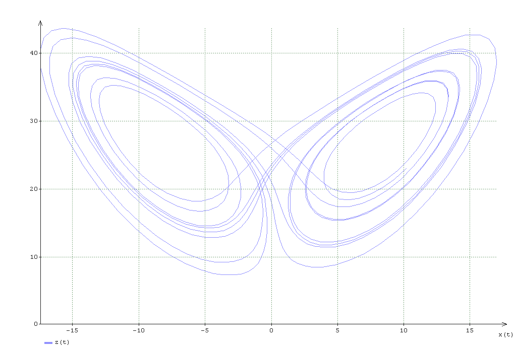
The results of the calculation on the phase plane z (x):

And y (x):

')
It seems that the curves are closed, but let's consider the result in more detail.
Taking the parameters for calculation from the article "Dynamic Lorenz system and computational experiment" :
The initial conditions, the parameters of the dynamic system, the accuracy of mathematical operations are 180 decimal places, the accuracy in the power series 1e-9, we get the following result at the point t = 6.827:


Derivative values:

It is easy to see that the results of the calculations are somewhat different from those stated in the article.
In addition, if we substitute the result from the article (the approximate values of the solutions found) into the original system of equations, we obtain the values of the derivatives that also differ from those indicated in the article:

I note that improving the accuracy of calculations (the number of decimal places taken into account and the accuracy in a power series) only leads to a narrowing of the region containing exact solutions. For example, when specifying the accuracy of 1e-55, the area at the point t = 6.827 narrows to .
.
Next, I decided to continue the calculation to the point t = 12.827 and consider the graph of the calculation results on the phase planes z (x):
And y (x):

The graphs clearly show that the curves are not closed. To be more precise, they are not closed in the first graphs either, just the scale in which the phase trajectories are displayed does not allow them to see the open point.
Thus, it is impossible to talk about any return of the trajectory to the vicinity of the starting point - this is stated in the article. And it is always necessary to draw conclusions on the basis of calculations with an eye to the calculation error (both methodical and computational).
Literature:
1. Bychkov Yu., Shcherbakov S. An analytical-numerical method for calculating dynamic systems. - St. Petersburg: Energoatomizdat, 2001.
The results of the calculation on the phase plane z (x):
And y (x):
')
It seems that the curves are closed, but let's consider the result in more detail.
Briefly about the calculation method used
The analytical-numerical method belongs to self-starting continuous methods of variable order with an adaptive procedure for selecting a step and with control of the levels of absolute maximum local and full calculation errors.
It is used to solve ordinary nonlinear nonautonomous non-stationary integrodifferential equations describing dynamic models of systems with deterministic influences.
When calculating the regular component of the desired solution is presented in the form of a Taylor series.
The result of applying an analytical-numerical method for solving systems of ordinary differential equations describing a model of a dynamic system is not only approximate solutions but also areas that are guaranteed to contain exact solutions.
That is, besides the very numerical value of the approximate solution, the result is the upper estimates of the maximum total calculation error at each calculation step:

Where - approximate solution (i-th phase coordinate);
 - unknown exact solution;
 - the upper estimate of the maximum total error in the calculation of the approximate solution;
It is used to solve ordinary nonlinear nonautonomous non-stationary integrodifferential equations describing dynamic models of systems with deterministic influences.
When calculating the regular component of the desired solution is presented in the form of a Taylor series.
The result of applying an analytical-numerical method for solving systems of ordinary differential equations describing a model of a dynamic system is not only approximate solutions but also areas that are guaranteed to contain exact solutions.
That is, besides the very numerical value of the approximate solution, the result is the upper estimates of the maximum total calculation error at each calculation step:
Where
- approximate solution (i-th phase coordinate); - unknown exact solution; - the upper estimate of the maximum total error in the calculation of the approximate solution;Taking the parameters for calculation from the article "Dynamic Lorenz system and computational experiment" :
The initial conditions, the parameters of the dynamic system, the accuracy of mathematical operations are 180 decimal places, the accuracy in the power series 1e-9, we get the following result at the point t = 6.827:
Derivative values:
It is easy to see that the results of the calculations are somewhat different from those stated in the article.
In addition, if we substitute the result from the article (the approximate values of the solutions found) into the original system of equations, we obtain the values of the derivatives that also differ from those indicated in the article:
I note that improving the accuracy of calculations (the number of decimal places taken into account and the accuracy in a power series) only leads to a narrowing of the region containing exact solutions. For example, when specifying the accuracy of 1e-55, the area at the point t = 6.827 narrows to
.Next, I decided to continue the calculation to the point t = 12.827 and consider the graph of the calculation results on the phase planes z (x):
And y (x):
The graphs clearly show that the curves are not closed. To be more precise, they are not closed in the first graphs either, just the scale in which the phase trajectories are displayed does not allow them to see the open point.
Thus, it is impossible to talk about any return of the trajectory to the vicinity of the starting point - this is stated in the article. And it is always necessary to draw conclusions on the basis of calculations with an eye to the calculation error (both methodical and computational).
Literature:
1. Bychkov Yu., Shcherbakov S. An analytical-numerical method for calculating dynamic systems. - St. Petersburg: Energoatomizdat, 2001.
Source: https://habr.com/ru/post/230647/
All Articles