Skip Lists: A Probabilistic Alternative to Balanced Trees
Gap lists are a data structure that can be used in place of balanced trees. Due to the fact that the balancing algorithm is probabilistic and not strict, inserting and deleting an element in the lists with gaps is much easier and much faster than in balanced trees.
Skip lists are a probabilistic alternative to balanced trees. They are balanced using a random number generator. Despite the fact that the lists with gaps have poor performance in the worst case, there is no such sequence of operations in which this would occur all the time (just like in the quick sort algorithm with a random selection of the reference element). It is very unlikely that this data structure will be significantly unbalanced (for example, for a dictionary larger than 250 elements, the probability that a search will take three times more than the expected time is less than one millionth).
')
Balancing a data structure is probably simpler than explicitly balancing. For many tasks, skip lists are a more natural representation of data than trees. Algorithms are simpler to implement and, in practice, faster than balanced trees. In addition, lists with gaps use memory very efficiently. They can be implemented in such a way that an average of approximately 1.33 pointer (or even less) falls on one element and does not require storage for each element of additional information about the balance or priority.
To search for an element in a linked list, we must look at each of its nodes:

If the list is kept sorted and every second node additionally contains a pointer to two nodes ahead, we need to look at no more than ⌈ n / 2⌉ + 1 nodes (where n is the length of the list):

Similarly, if now every fourth node contains a pointer to four nodes forward, then you need to view no more than ⌈ n / 4⌉ + 2 nodes:

If every 2 i- th node contains a pointer to 2 i nodes ahead, then the number of nodes that need to be viewed will decrease to ⌈log 2 n ⌉, and the total number of pointers in the structure will only double:
This data structure can be used for quick lookups, but inserting and deleting nodes will be slow.
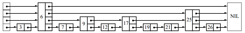
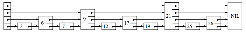
We call a node containing k pointers to the front elements, a node of level k . If every 2 i- th node contains a pointer to 2 i nodes ahead, then the levels are distributed as follows: 50% of the nodes - level 1, 25% - level 2, 12.5% - level 3, etc. But what happens if the levels of nodes are chosen randomly, in the same proportions? For example:
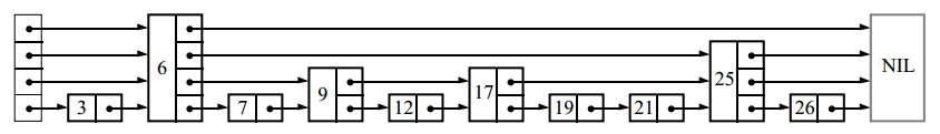
Pointer number i of each node will refer to the next node of level i or more, and not exactly 2 i -1 nodes forward, as it was before. Insertions and deletions will require only local changes; the level of a node chosen randomly when it is inserted will never change. In case of unsuccessful assignment of levels, performance may turn out to be low, but we will show that such situations are rare. Due to the fact that these data structures are connected lists with additional pointers to skip intermediate nodes, I call them lists with gaps.
Operations
We describe the algorithms for searching, inserting and deleting elements in the dictionary, implemented on lists with gaps. The search operation returns a value for the specified key or signals that the key was not found. The insert operation associates the key with the new value (and creates the key if it was not there before). The delete operation deletes the key. Also in this data structure, you can easily add additional operations, such as “finding the minimum key” or “finding the next key”.
Each element of the list is a node, the level of which was chosen randomly during its creation, regardless of the number of elements that were already there. The node of level i contains i pointers to the various elements ahead, indexed from 1 to i . We may not store the node level in the node itself. The number of levels is limited by the pre-selected constant MaxLevel . Let's call the list level the maximum level of a node in this list (if the list is empty, then the level is 1). The title of the list (in the pictures on the left) contains pointers to levels 1 through MaxLevel . If there are no elements of this level yet, then the pointer value is a special element of NIL.
Initialization
Create an NIL element, the key of which is larger than any key that may ever appear in the list. The NIL element will complete all lists with gaps. The list level is 1, and all pointers from the header refer to NIL.
Item Search
Starting with the highest level indicator, we move forward along the indexes until they refer to an element that does not exceed the desired one. Then we go down one level below and again move by the same rule. If we have reached level 1 and can’t go any further, then we are just before the element we are looking for (if there is one).
Search (list, searchKey)
x: = list → header
# loop invariant: x → key <searchKey
for i: = list → level downto 1 do
while x → forward [i] → key <searchKey do
x: = x → forward [i]
# x → key <searchKey ≤ x → forward [1] → key
x: = x → forward [1]
if x → key = searchKey then return x → value
else return failure
Insert and delete item
To insert or delete a node, use the search algorithm to find all elements before the one being inserted (or deleted), then update the corresponding pointers:
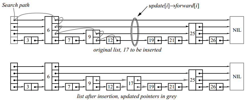
In this example, we inserted a level 2 element.
Insert (list, searchKey, newValue)
local update [1..MaxLevel]
x: = list → header
for i: = list → level downto 1 do
while x → forward [i] → key <searchKey do
x: = x → forward [i]
# x → key <searchKey ≤ x → forward [i] → key
update [i]: = x
x: = x → forward [1]
if x → key = searchKey then x → value: = newValue
else
lvl: = randomLevel ()
if lvl> list → level then
for i: = list → level + 1 to lvl do
update [i]: = list → header
list → level: = lvl
x: = makeNode (lvl, searchKey, value)
for i: = 1 to level do
x → forward [i]: = update [i] → forward [i]
update [i] → forward [i]: = x
Delete (list, searchKey)
local update [1..MaxLevel]
x: = list → header
for i: = list → level downto 1 do
while x → forward [i] → key <searchKey do
x: = x → forward [i]
update [i]: = x
x: = x → forward [1]
if x → key = searchKey then
for i: = 1 to list → level do
if update [i] → forward [i] then x then break
update [i] → forward [i]: = x → forward [i]
free (x)
while list → level> 1 and list → header → forward [list → level] = NIL do
list → level: = list → level - 1
To memorize elements before being inserted (or deleted), the update array is used. The update [i] element is a pointer to the rightmost node, level i or higher, from among those to the left of the update location.
If a randomly selected level of the inserted node is greater than the level of the entire list (i.e. if there are no nodes with that level yet), increase the list level and initialize the corresponding elements of the update array with pointers to the header. After each deletion, we check whether we deleted the node with the maximum level and, if so, reduce the list level.
Level number generation
Previously, we cited the distribution of node levels in the case where half of the nodes containing the level indicator i also contained a pointer to a node of level i +1. To get rid of the magic constant 1/2, we denote by p the fraction of nodes of level i containing a pointer to nodes of level i + i. The level number for the new vertex is generated randomly according to the following algorithm:
randomLevel ()
lvl: = 1
# random () returns a random number in the half-interval [0 ... 1)
while random () <p and lvl <MaxLevel do
lvl: = lvl + 1
return lvl
As you can see, the number of elements in the list does not participate in the generation.
What level to start looking for? Definition of L (n)
In the list with gaps of 16 elements generated at p = 1/2, it may turn out that it contains 9 elements of level 1, 3 elements of level 2, 3 elements of level 3 and 1 element of level 14 (this is unlikely, but possible) . How to deal with this? If we use the standard algorithm and search from level 14, we will do a lot of useless work.
Where better to start the search? Our research has shown that it is best to start the search from the L level, where we expect 1 / p nodes. This will happen when L = log 1 / p n . For convenience of further reasoning, we denote the function log 1 / p n as L ( n ).
There are several ways to solve problems with nodes of unexpectedly large level:
- Do not bathe (orig. Don't worry, be happy). Just start the search from the largest level on the list. As we will see later, the probability that the list level of n elements turns out to be much higher than L (n) is very small. This solution adds only a small constant to the expected search time. This approach is used in the algorithms given above.
- Use less space than needed. Although an element can contain 14 pointers, we do not have to use all 14. We can use only L (n) of them. There are several ways to implement this, but they all complicate the algorithm and do not lead to a noticeable increase in performance. This method is not recommended for use.
- Fix the cube. If a level is generated that is greater than the maximum node level in the list, then we simply assume that it is exactly 1 more. In theory, and it seems, in practice, this works well. But with this approach, we completely lose the opportunity to analyze the complexity of the algorithms, since the node level is no longer completely random. Programmers are free to use this method, but it is better for theoreticians to avoid it.
MaxLevel selection
Since the expected number of levels is L (n), it is best to choose MaxLevel = L ( N ), where N is the maximum number of items in the list with gaps. For example, if p = 1/2, then MaxLevel = 16 is suitable for lists containing less than 2 16 elements.
Algorithm Analysis
In the search, insert and delete operations, the most time is spent searching for a suitable element. For the insertion and deletion, additional time is necessary proportional to the level of the node being inserted or removed. The search time for an element is proportional to the number of nodes passed in the search process, which, in turn, depends on the distribution of their levels.
Probabilistic philosophy
The list structure with gaps is determined only by the number of elements in this list and the values of the random number generator. The sequence of operations with which the list is obtained is not important. We assume that the user does not have access to the node levels, otherwise, he can make the algorithm work in the worst possible time by deleting all nodes whose level is different from 1.
For sequential operations on the same data structure, their execution times are not independent random variables; two consecutive searches for the same item will take exactly the same time.
Analysis of the expected search time
Consider the search path from the end, i.e. let's move up and left. Although the levels of nodes in the list are known and fixed at the time of the search, we assume that the node level is determined only when we met it when moving from the end.
At any given point on the road we are in this situation:

We look at the i- th pointer of the node x and do not know about the levels of the nodes to the left of x . Also, we do not know the exact level of x , but it must be at least i . Suppose that x is not a list header (this is equivalent to assuming that the list expands indefinitely to the left). If level x is i , then we are in situation b . If the level x is greater than i , then we are in a situation c . The probability that we are in situation c is p . Every time this happens, we go up one level. Let C ( k ) be the expected length of the search return path, at which we moved up k times:
C (0) = 0
C ( k ) = (1- p ) ( path length in situation b ) + p ( path length in situation c )
Simplify:
C ( k ) = (1- p ) (1 + C ( k )) + p (1 + C ( k -1))
C ( k ) = 1 + C ( k ) - p ⋅ C ( k ) + p ⋅ C ( k -1)
C ( k ) = 1 / p + C ( k - 1)
C ( k ) = k / p
Our suggestion that the list is endless is pessimistic. When we reach the leftmost element, we simply move up all the time, not moving left. This gives us the upper bound ( L ( n ) - 1) / p of the expected path length from the node with level 1 to the node with level L ( n ) in the list of n items.
We use these reasonings to get to the node of level L ( n ), but other reasoning is used for the rest of the way. The number of remaining moves to the left is limited by the number of nodes having a level of L ( n ), or higher in the entire list. The most likely number of such nodes is 1 / p .
We also move up from the L ( n ) level to the maximum level in the list. The probability that the maximum list level is greater than k is 1- (1-p k ) n , which is not greater than np k . We can calculate that the expected maximum level is not more than L ( n ) + 1 / (1- p ). Putting it all together, we get that the expected length of the search path for a list of n items
<= L ( n ) / p + 1 / (1- p ),
or O (log n ).
Number of comparisons
We have just calculated the length of the path traveled by the search. The required number of comparisons per unit is greater than the length of the path (the comparison occurs at each step of the path).
Probabilistic analysis
We can consider the probability distribution of various search path lengths. Probabilistic analysis is somewhat more complicated (it is at the very end of the original article). With it, we can estimate from above the probability that the length of the search path will exceed the expected one more than by a specified number of times. Analysis results:
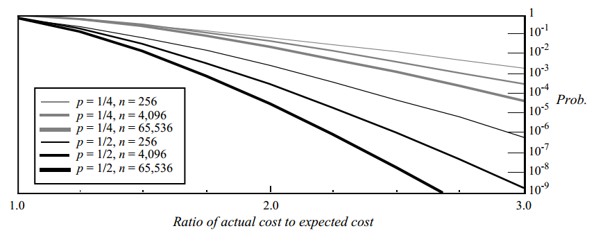
Here is a graph of the upper limit of the probability that the operation will take significantly longer than expected. On the vertical axis, the probability is set aside that the length of the search path will be more than the expected path length by the number of times plotted on the horizontal axis. For example, with p = 1/2 and n = 4096, the probability that the resulting path is three times longer than expected is less than 1/200 000 000.
Choice p
The table shows the normalized search times and the amount of required memory for different values of p :
| p | Normalized search time (i.e. normalized L ( n ) / p ) | Average number of pointers per node (i.e. 1 / (1 - p )) |
|---|---|---|
| 1/2 | one | 2 |
| 1 / e | 0.94 ... | 1.58 ... |
| 1/4 | one | 1.33 ... |
| 1/8 | 1.33 ... | 1.14 ... |
| 1/16 | 2 | 1.07 ... |
Decreasing p increases the spread of operation time. If 1 / p is a power of two, then it is convenient to generate a level number from a stream of random bits (to generate on average, (log 2 1 / p ) / (1- p ) random bits are required). Since there are overheads related to L ( n ) (but not to L ( n ) / p ), the choice of p = 1/4 (instead of 1/2) slightly reduces the constant in the complexity of the algorithm. We recommend choosing p = 1/4, but if the spread of the operation time is more important for you than the speed, then choose 1/2.
Multiple operations
The expected total time of the sequence of operations is equal to the sum of the expected times for each operation in the sequence. Thus, the expected time for any sequence of m operations in the data structure of n elements is O ( m * log n ). However, the pattern of search operations affects the distribution of the actual time of the entire sequence of operations.
If we search for the same element in the same data structure, then both operations will take exactly the same time. Thus, the variance (spread) of the total time will be four times the variance of a single search operation. If the search times for two elements are independent random variables, then the variance of the total time is equal to the sum of the variances of the times of individual operations. Finding the same element again and again maximizes variance.
Performance tests
Let's compare the performance of lists with gaps with other data structures. All implementations have been optimized for maximum performance:
| Data structure | Search | Insert | Deletion |
|---|---|---|---|
| lists with gaps | 0.051 ms (1.0) | 0.065 ms (1.0) | 0.059 ms (1.0) |
| non-recursive AVL trees | 0.046 ms (0.91) | 0.10 ms (1.55) | 0.085 ms (1.46) |
| recursive 2-3 trees | 0.054 ms (1.05) | 0.21 ms (3.2) | 0.21 ms (3.65) |
| Self-regulating trees: | |||
| top-down splaying | 0.15 ms (3.0) | 0.16 ms (2.5) | 0.18 ms (3.1) |
| bottom-up splaying | 0.49 ms (9.6) | 0.51 ms (7.8) | 0.53 ms (9.0) |
Tests were performed on a Sun-3/60 machine and were performed on data structures containing 2 16 elements. Values in brackets - time, relative to lists with gaps (in times). For tests of insertion and deletion of elements, the time spent on managing the memory was not taken into account (for example, for C-calls of malloc and free).
Note that lists with gaps require more comparison operations than other data structures (the algorithms given above require on average L ( n ) / p + 1 / (1 + p ) operations). When using real numbers as keys, operations in lists with gaps turned out to be a little slower than in the non-recursive implementation of the AVL tree, and searching in lists with gaps was a little slower than searching in 2-3 trees (however, inserting and deleting in the lists with gaps were faster than in the recursive implementation of 2-3 trees). If the comparison operations are very expensive, you can modify the algorithm so that the key you are looking for will not be compared with the key of other nodes more than once per node. When p = 1/2, the upper limit of the number of comparisons is 7/2 + 3/2 * log 2 n .
Uneven distribution of requests
Self-regulating trees can adapt to the uneven distribution of requests. Since lists with gaps are faster than self-regulating trees a fairly large number of times, self-regulating trees are faster only with some very uneven distribution of requests. We could try to develop self-regulating lists with gaps, however, we did not see any practical sense in this and did not want to spoil the simplicity and performance of the original implementation. If the application expects non-uniform queries, then using self-regulating trees or adding caching will be preferable.
Conclusion
From a theoretical point of view, lists with gaps are not needed. Balanced trees can do the same operations and have a good difficulty at worst (as opposed to lists with gaps). However, the implementation of balanced trees is a difficult task and, as a result, they are rarely implemented in practice, except as lab work in universities.
Gap lists are a simple data structure that can be used instead of balanced trees in most cases. Algorithms are very easy to implement, extend and modify. Regular implementations of operations on gaps with lists are about as fast as highly optimized implementations on balanced trees and are significantly faster than ordinary, non-highly optimized implementations.
Source: https://habr.com/ru/post/230413/
All Articles