Probabilistic models: LDA, part 2
We continue the conversation. Last time, we took the first step in the transition from the naive Bayes classifier to the LDA: we removed the need to mark up the training set from the naive Bayes, making it a clustering model that you can train with the EM algorithm. Today, I no longer have any excuses - I’ll have to talk about the LDA model itself and show how it works. Once we talked about LDA in this blog, but then the story was very short and without very significant details. I hope that this time it will be possible to tell more and more clearly.

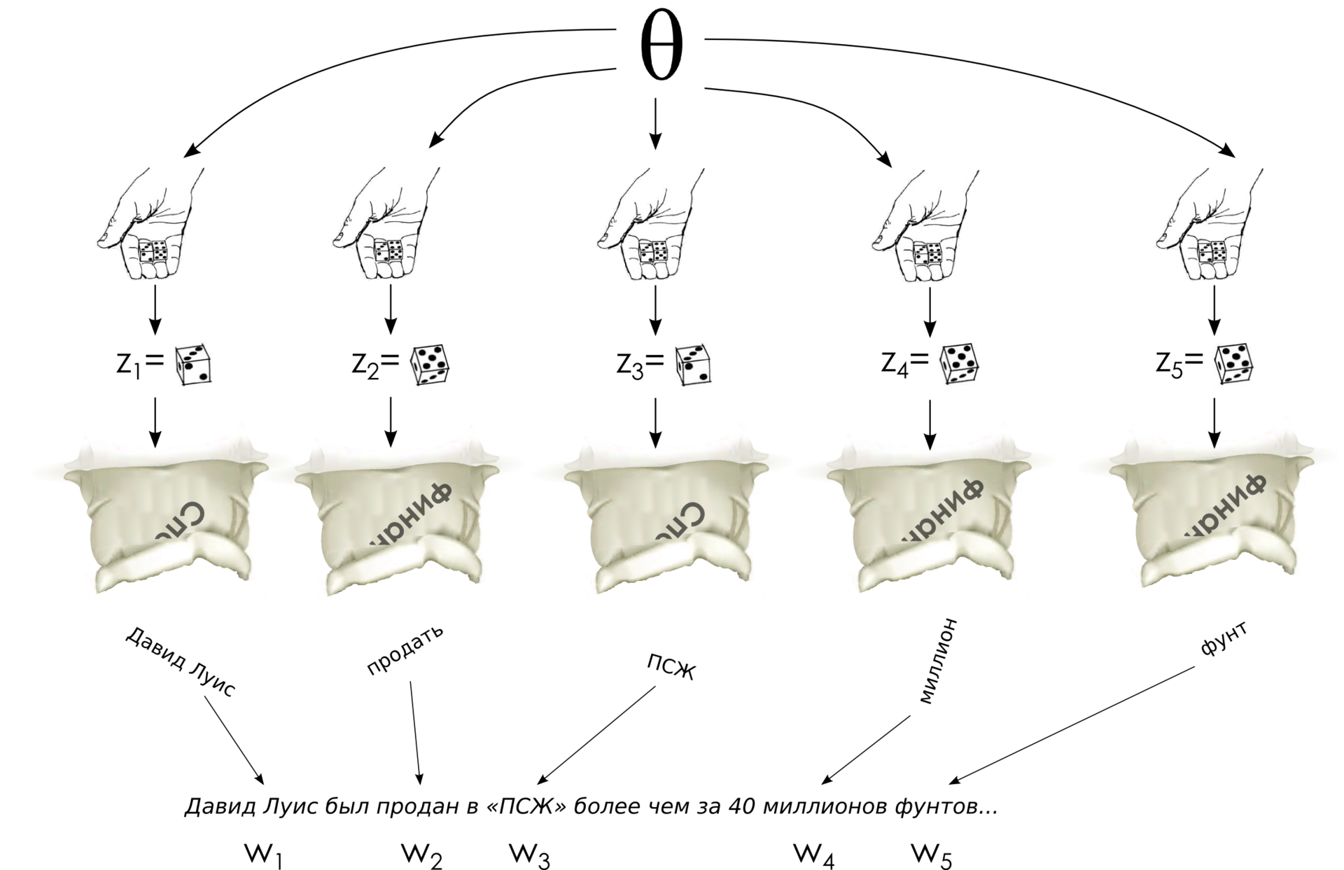
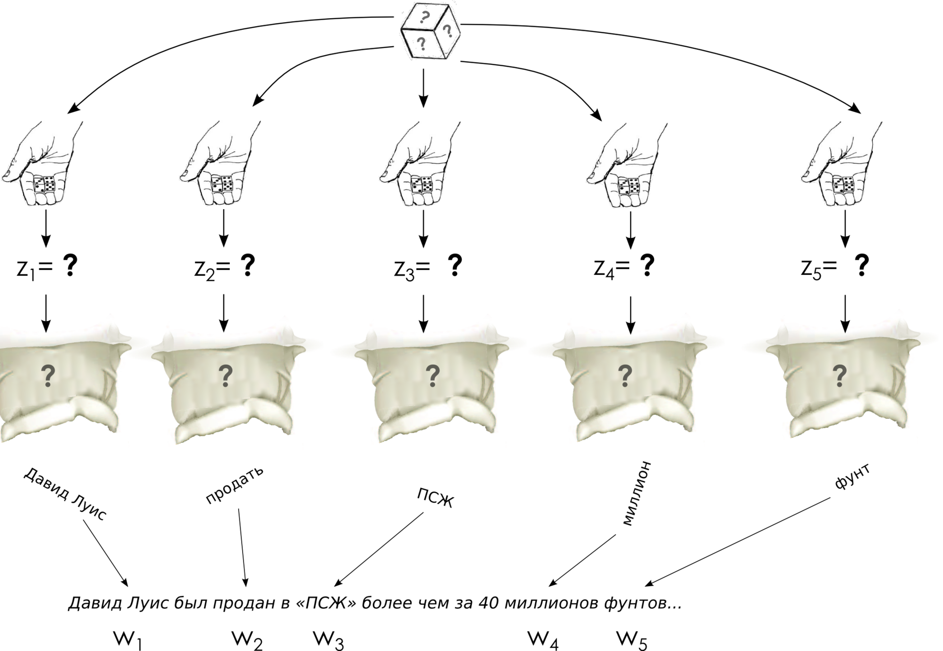
So, we start talking about the LDA. Let me remind you that the main goal of our generalization is to ensure that the document is not rigidly tied to one topic, and the words in the documents could come from several topics at once. What does this mean in (mathematical) reality? This means that the document is a mixture of topics, and each word can be generated from one of the topics in this mixture. Simply put, we first throw a dice-document, defining a theme for each word , and then pull the word out of the corresponding bag.
Thus, the basic intuition of the model looks like this:
')
Since intuition is the most important thing, and here it is not the simplest, I will repeat the same thing again in other words, now a little more formally. It is convenient to understand and represent probabilistic models in the form of generative processes, when we consistently describe how one unit of data is generated, introducing along the way all probabilistic assumptions that we make in this model. Accordingly, the generating process for the LDA must consistently describe how we generate each word of each document. And this is how it happens (hereinafter I will assume that the length of each document is set — you can also add it to the model, but usually this does not give anything new):
Here, the process of choosing a word with the data θ and φ should already be clear to the reader - we throw a die for each word and choose the topic of the word, then pull the word out of the corresponding bag:
In the model, it remains to explain only where these θ and φ come from and what the expression ; it also explains why this is called Dirichlet allocation.
Johann Peter Gustav Lejeun Dirichlet was not so much concerned with the theory of probability; he mainly specialized in mathematical analysis, number theory, Fourier series, and other similar mathematics. In probability theory, he was not so often seen, although, of course, his results in probability theory would make a brilliant career in modern mathematics (the trees were greener, the sciences were less studied, and, in particular, the mathematical Klondike was also not exhausted). However, in his studies of mathematical analysis, Dirichlet, in particular, managed to take this classical integral, which as a result was called the Dirichlet integral:
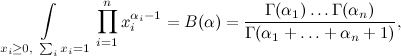
where Γ (α i ) is a gamma function, the continuation of factorial (for natural numbers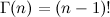 ). Dirichlet himself derived this integral for the needs of celestial mechanics, then Liouville found a simpler conclusion, which was generalized to more complex forms of integrand functions, and wrap everything up.
The Dirichlet distribution, motivated by the Dirichlet integral, is the distribution on the ( n -1) -dimensional vector x 1 , x 2 , ..., x n -1 , defined as follows:
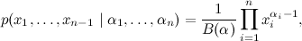
Where , and the distribution is given only on the ( n -1) -dimensional simplex, where x i > 0. From the Dirichlet integral in it appeared normalization constant. And the meaning of the Dirichlet distribution is quite elegant - it is a distribution on distributions . Look - as a result of vector sketching over the Dirichlet distribution, a vector with non-negative elements is obtained, the sum of which is equal to one ... ba, and this is a discrete probability distribution, actually a dishonest cube with n edges.
Of course, this is not the only possible class of distributions on discrete probabilities, but the Dirichlet distribution also has a number of other attractive properties. The main thing is that it is a conjugate prior distribution for that same dishonest cube; I will not explain in detail what this means (perhaps later), but, in general, it is reasonable to take the Dirichlet distribution as an a priori distribution in probabilistic models, when you want to get an unfair cube as a variable.
It remains to discuss what, in fact, will be obtained for different values of α i . First of all, let us immediately confine ourselves to the case when all α i are the same - we a priori have no reason to prefer some topics to others, we at the beginning of the process still do not know where which topics stand out. Therefore, our distribution will be symmetrical.
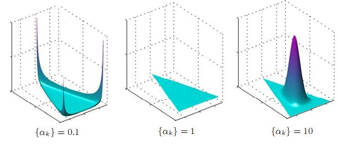
What does it mean - the distribution on the simplex? What does it look like? Let's draw several such distributions - we can draw a maximum in three-dimensional space, so the simplex will be two-dimensional - a triangle, in other words, - and the distribution will be over this triangle (the picture is taken from here ; in principle, you understand what it is about, but very interesting why Uniform (0,1) is signed under Pandora's box - if anyone understands, tell me :)):
But similar distributions in two-dimensional format, in the form of heatmap (as they can be drawn, explained, for example, here ); however, here 0.1 would be completely invisible, so I replaced it with 0.995:
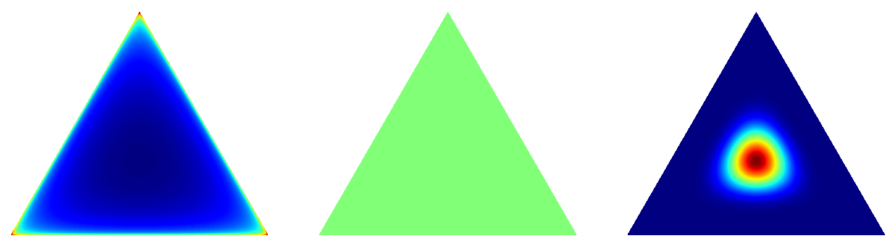
And this is what happens: if α = 1, we get a uniform distribution (which is logical - then all the powers in the density function are zero). If α is greater than one, then with a further increase in α, the distribution becomes more and more concentrated in the center of the simplex. For large α, we will almost always get almost completely honest cubes. But the most interesting thing here is what happens when α is less than one — in this case, the distribution focuses on the corners and edges / sides of the simplex! In other words, for small α, we will obtain sparse cubes — distributions in which almost all probabilities are equal or close to zero, and only a small part of them are essentially nonzero. This is exactly what we need - and in the document we would like to see some essentially expressed topics, and the topic would be well enough to clearly outline a relatively small subset of words. Therefore, in LDA, α and β hyper parameters are usually less than one, usually α = 1 / T (inverse to the number of topics) and β = Const / W (a constant like 50 or 100 divided by the number of words).
Disclaimer: my presentation follows the simplest and most straightforward approach to the LDA, I try to convey a general understanding of the model with large strokes. In fact, of course, there are more detailed studies on how to choose the α and β hyperparameters, what they give and what they lead to; in particular, hyperparameters are not at all required to be symmetrical. See, for example, the article Wallach, Nimho, McCallum " Rethinking LDA: Why Priors Matter ".
Let's summarize. We have already explained all parts of the model — the Dirichlet a priori distribution produces dice-documents and sack-themes, throwing a cube-document determines its own theme for each word, and then the word itself is selected from the corresponding sack-theme. Formally speaking, it turns out that the graphical model looks like this:
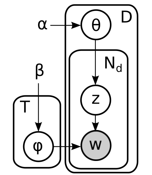
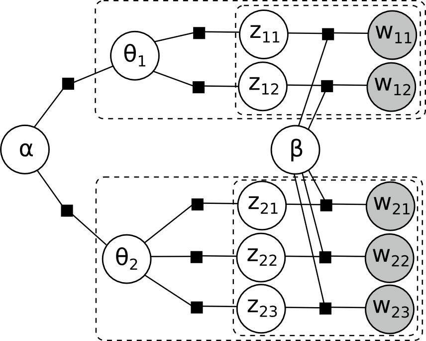
Here the inner plate corresponds to the words of one document, and the outer plate corresponds to the documents in the body. No need to be deceived by the external simplicity of this picture, there are more than enough cycles here; here, for example, a fully expanded factor graph for two documents, one of which has two words, and the other three:
And the joint probability distribution, it turns out, is factorized as follows:

What is the task of learning the LDA model now? It turns out that only words are given to us, nothing is given any more, and we must somehow train all-all-all these parameters. The task looks very scary - nothing is known and everything must be pulled out of the set of documents:
Nevertheless, it is solved with the help of the very methods of approximate inference that we talked about earlier. Next time we will talk about how to solve this problem, apply the Gibbs sampling method (see one of the previous installations ) to the LDA model and derive the update equations for variables z w ; we will see that in fact all this terrible mathematics is not so terrible at all, and the LDA is quite understandable not only conceptually, but also algorithmically.
LDA: intuition
So, we start talking about the LDA. Let me remind you that the main goal of our generalization is to ensure that the document is not rigidly tied to one topic, and the words in the documents could come from several topics at once. What does this mean in (mathematical) reality? This means that the document is a mixture of topics, and each word can be generated from one of the topics in this mixture. Simply put, we first throw a dice-document, defining a theme for each word , and then pull the word out of the corresponding bag.
Thus, the basic intuition of the model looks like this:
- there are themes in the world (unknown in advance) that reflect what parts of a document can be about;
- each topic is a probability distribution in words, i.e. a bag of words from which you can with different probabilities pull out different words;
- each document is a mixture of topics, i.e. probability distribution on topics, a die that can be thrown;
- The process of generating each word is to first select a topic in the distribution corresponding to the document, and then select a word from the distribution corresponding to that topic.
')
Since intuition is the most important thing, and here it is not the simplest, I will repeat the same thing again in other words, now a little more formally. It is convenient to understand and represent probabilistic models in the form of generative processes, when we consistently describe how one unit of data is generated, introducing along the way all probabilistic assumptions that we make in this model. Accordingly, the generating process for the LDA must consistently describe how we generate each word of each document. And this is how it happens (hereinafter I will assume that the length of each document is set — you can also add it to the model, but usually this does not give anything new):
- for each topic t :
- choose the vector φ t (distribution of words in the topic) according to the distribution
 ;
;
- choose the vector φ t (distribution of words in the topic) according to the distribution
- for each document d :
- choose vector - the vector of "severity" of each topic in this document;
- for each word in the document w :
- select a topic z w by distribution
 ;
; - choose a word
 with probabilities given in β.
- select a topic z w by distribution
- choose vector
Here, the process of choosing a word with the data θ and φ should already be clear to the reader - we throw a die for each word and choose the topic of the word, then pull the word out of the corresponding bag:
In the model, it remains to explain only where these θ and φ come from and what the expression
; it also explains why this is called Dirichlet allocation.What does Dirichlet have to do with it?
Johann Peter Gustav Lejeun Dirichlet was not so much concerned with the theory of probability; he mainly specialized in mathematical analysis, number theory, Fourier series, and other similar mathematics. In probability theory, he was not so often seen, although, of course, his results in probability theory would make a brilliant career in modern mathematics (the trees were greener, the sciences were less studied, and, in particular, the mathematical Klondike was also not exhausted). However, in his studies of mathematical analysis, Dirichlet, in particular, managed to take this classical integral, which as a result was called the Dirichlet integral:
where Γ (α i ) is a gamma function, the continuation of factorial (for natural numbers
). Dirichlet himself derived this integral for the needs of celestial mechanics, then Liouville found a simpler conclusion, which was generalized to more complex forms of integrand functions, and wrap everything up.The Dirichlet distribution, motivated by the Dirichlet integral, is the distribution on the ( n -1) -dimensional vector x 1 , x 2 , ..., x n -1 , defined as follows:
Where
, and the distribution is given only on the ( n -1) -dimensional simplex, where x i > 0. From the Dirichlet integral in it appeared normalization constant. And the meaning of the Dirichlet distribution is quite elegant - it is a distribution on distributions . Look - as a result of vector sketching over the Dirichlet distribution, a vector with non-negative elements is obtained, the sum of which is equal to one ... ba, and this is a discrete probability distribution, actually a dishonest cube with n edges.Of course, this is not the only possible class of distributions on discrete probabilities, but the Dirichlet distribution also has a number of other attractive properties. The main thing is that it is a conjugate prior distribution for that same dishonest cube; I will not explain in detail what this means (perhaps later), but, in general, it is reasonable to take the Dirichlet distribution as an a priori distribution in probabilistic models, when you want to get an unfair cube as a variable.
It remains to discuss what, in fact, will be obtained for different values of α i . First of all, let us immediately confine ourselves to the case when all α i are the same - we a priori have no reason to prefer some topics to others, we at the beginning of the process still do not know where which topics stand out. Therefore, our distribution will be symmetrical.
What does it mean - the distribution on the simplex? What does it look like? Let's draw several such distributions - we can draw a maximum in three-dimensional space, so the simplex will be two-dimensional - a triangle, in other words, - and the distribution will be over this triangle (the picture is taken from here ; in principle, you understand what it is about, but very interesting why Uniform (0,1) is signed under Pandora's box - if anyone understands, tell me :)):
But similar distributions in two-dimensional format, in the form of heatmap (as they can be drawn, explained, for example, here ); however, here 0.1 would be completely invisible, so I replaced it with 0.995:
And this is what happens: if α = 1, we get a uniform distribution (which is logical - then all the powers in the density function are zero). If α is greater than one, then with a further increase in α, the distribution becomes more and more concentrated in the center of the simplex. For large α, we will almost always get almost completely honest cubes. But the most interesting thing here is what happens when α is less than one — in this case, the distribution focuses on the corners and edges / sides of the simplex! In other words, for small α, we will obtain sparse cubes — distributions in which almost all probabilities are equal or close to zero, and only a small part of them are essentially nonzero. This is exactly what we need - and in the document we would like to see some essentially expressed topics, and the topic would be well enough to clearly outline a relatively small subset of words. Therefore, in LDA, α and β hyper parameters are usually less than one, usually α = 1 / T (inverse to the number of topics) and β = Const / W (a constant like 50 or 100 divided by the number of words).
Disclaimer: my presentation follows the simplest and most straightforward approach to the LDA, I try to convey a general understanding of the model with large strokes. In fact, of course, there are more detailed studies on how to choose the α and β hyperparameters, what they give and what they lead to; in particular, hyperparameters are not at all required to be symmetrical. See, for example, the article Wallach, Nimho, McCallum " Rethinking LDA: Why Priors Matter ".
LDA: graph, co-distribution, factorization
Let's summarize. We have already explained all parts of the model — the Dirichlet a priori distribution produces dice-documents and sack-themes, throwing a cube-document determines its own theme for each word, and then the word itself is selected from the corresponding sack-theme. Formally speaking, it turns out that the graphical model looks like this:
Here the inner plate corresponds to the words of one document, and the outer plate corresponds to the documents in the body. No need to be deceived by the external simplicity of this picture, there are more than enough cycles here; here, for example, a fully expanded factor graph for two documents, one of which has two words, and the other three:
And the joint probability distribution, it turns out, is factorized as follows:
What is the task of learning the LDA model now? It turns out that only words are given to us, nothing is given any more, and we must somehow train all-all-all these parameters. The task looks very scary - nothing is known and everything must be pulled out of the set of documents:
Nevertheless, it is solved with the help of the very methods of approximate inference that we talked about earlier. Next time we will talk about how to solve this problem, apply the Gibbs sampling method (see one of the previous installations ) to the LDA model and derive the update equations for variables z w ; we will see that in fact all this terrible mathematics is not so terrible at all, and the LDA is quite understandable not only conceptually, but also algorithmically.
Source: https://habr.com/ru/post/230103/
All Articles