Lorentz's dynamic system and computational experiment

This post is a continuation of my article [1] on Habrahabr about Lorenz attractor. Here we consider the method of constructing approximate solutions of the corresponding system, paying attention to the software implementation.

The dynamical system of Lorentz is an autonomous system of ordinary differential equations of the third order.
')


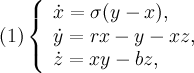
Where , r and b are positive numbers. To study the behavior of system solutions, one usually takes the classical values ​​of the system parameters, i.e.



As it was noted in the article [1], in this case, the instability of its solutions on the attractor takes place in system (1). In fact, this makes incorrect the application of classical numerical methods on large intervals of time (and on such intervals the limiting sets of dynamic systems are constructed). One of the ways to overcome this problem is the transition to high-precision calculations, but this approach puts the researcher in a rigid framework: first, a small degree of freedom to reduce the error (changing the step size integration and accuracy of the representation of a real number to control the computational process), secondly, a large amount of computation for very small .

Another solution to this problem may be the use of the power series method. In [2], a modification of this method was described for dynamic systems of the form (1), which makes it possible to quickly determine the expansion coefficients



as



where are the coefficients , and determined by the initial conditions; also obtained length (step) segment convergence series (2):



if a then otherwise ,

- any positive number.

Note that the scheme for obtaining the length of the convergence segment of power series given in [2] can be transferred by analogy to other third-order dynamic systems with nonlinearities of the form (1) (for example, a system describing the behavior of a self-developing market economy [3, p. 261]) .

Despite the fact that all trajectories of system (1) are limited and its right-hand side is everywhere analytic, the initial computational experiment showed that the radius of convergence of series (2) is limited and depends on the choice of initial conditions. Therefore, in the described way, we can get only a part of the trajectory. The procedure for constructing an arc of a trajectory at any time interval consists in matching the portions of the trajectory that make up the desired solution, on which the series (2) converge. The integration error accumulated during the transition from the arc to the arc of the trajectory due to the error in finding the current approximate solution can be controlled by varying the accuracy expansions in power series. The use of high-precision calculations allows us to continue the solutions for very long periods of time, since impossible to make arbitrarily small due to limitations on machine epsilon.

By the formulas (3) we calculate , and to such a value i for which the estimate holds



It is clear that we still cannot avoid a significant accumulation of integration error over long time intervals, so we will implement high-precision floating-point calculations based on the GNU MPFR Library , more precisely, the C ++ MPFR library interface for working with real numbers of arbitrary precision - MPFR C ++ . It is convenient because it has the mpreal class with overloaded arithmetic operations and friendly mathematical functions. To install the library in Ubuntu Linux run

sudo apt-get install libmpfrc++-dev 

In addition to the libmpfr-dev package, package managers will also pull libgmp-dev. This is the GNU Multiple Precision Arithmetic Library or GMP devel-package of the library (MPFR is its extension).

Consider the example code in C ++ calculating the values ​​of the phase coordinates at a finite point in time, as well as checking the values ​​found.

 #include <iostream> #include <vector> using namespace std; #include <mpreal.h> using namespace mpfr; //     #define eps_c "1e-50" //     #define sigma 10 #define r 28 #define b 8/(mpreal)3 //       #define prec 180 //   : 1 -    , 0 -   #define FL_CALC 1 //     #define step_t "0.02" //        mpreal get_delta_t(mpreal &alpha0, mpreal &beta0, mpreal &gamma0) { mpreal h2 = (mpfr::max)((mpfr::max)(fabs(alpha0), fabs(beta0)), fabs(gamma0)), h1 = (mpfr::max)((mpfr::max)(2*sigma, r+2*h2+1), b+2*h2+1); mpreal h3 = h2 >= 1 ? h1 * h2 : (mpfr::max)((mpfr::max)(2*sigma, r+2), b+1); return 1/(h3 + "1e-10"); } //          // x, y  z -   ; T -   ; // way -   : 1 -   , -1 -    void calc(mpreal &x, mpreal &y, mpreal &z, mpreal T, int way = 1) { cout << "\n   :\n\ndx/dt = " << sigma*(yx) << "\ndy/dt = " << r*xyx*z << "\ndz/dt = " << x*yb*z << endl; mpreal t = 0, delta_t, L, p, s1, s2; bool fl_rp; do { if(FL_CALC) delta_t = get_delta_t(x, y, z); else delta_t = step_t; t += delta_t; if(t < T) fl_rp = true; else if(t > T) { delta_t -= tT; fl_rp = false; } else fl_rp = false; vector<mpreal> alpha, beta, gamma; alpha.push_back(x); beta.push_back(y); gamma.push_back(z); int i = 0; L = sqrt(alpha[0]*alpha[0] + beta[0]*beta[0] + gamma[0]*gamma[0]); p = way * delta_t; while(L > eps_c) { //      s1 = s2 = 0; for(int j = 0; j <= i; j++) { s1 += alpha[j] * gamma[ij]; s2 += alpha[j] * beta[ij]; } alpha.push_back(sigma*(beta[i] - alpha[i])/(i+1)); beta.push_back((r*alpha[i] - beta[i] - s1)/(i+1)); gamma.push_back((s2 - b*gamma[i])/(i+1)); i++; x += alpha[i] * p; y += beta[i] * p; z += gamma[i] * p; L = fabs(p) * sqrt(alpha[i]*alpha[i] + beta[i]*beta[i] + gamma[i]*gamma[i]); p *= way * delta_t; } } while(fl_rp); cout << "\n    :\nx = " << x.toString() << "\ny = " << y.toString() << "\nz = " << z.toString() << endl; cout << "\n :\n\ndx/dt = " << sigma*(yx) << "\ndy/dt = " << r*xyx*z << "\ndz/dt = " << x*yb*z << endl; } int main() { mpreal::set_default_prec(prec); cout << "  = " << machine_epsilon() << endl; mpreal T; cout << "\n    > "; cin >> T; mpreal x, y, z; cout << "\nx0 > "; cin >> x; cout << "y0 > "; cin >> y; cout << "z0 > "; cin >> z; cout << endl; calc(x, y, z, T); cout << "\n\n***   ***\n"; calc(x, y, z, T, -1); return 0; } 

To compile the lorenz.cpp file with this code, run the following

 g++ lorenz.cpp -std=gnu++11 -lmpfr -lgmp -o lorenz 

As can be seen from the program listing, vectors from the STL library are used to store the values ​​of the coefficients of power series. It was assumed that the number of bits under the mantissa of a real number is 180. The exponential variation range is by default from before (on 32-bit platforms). Machine_epsilon () definition function for machine epsilon was used to find out its value for a given representation of a real number. In this case



We present the results of a computational experiment. As initial conditions, we take values ​​close to the Lorentz attractor:



The length of time at which the calculations were made, - . Initially, the accuracy of the assessment of the total member of the series was taken to be . This is enough to get a result.

;

derivatives:



(decreasing value , coordinate values ​​will not change). In this case, you can take real numbers with less memory.

The values ​​of the derivatives, as well as the values ​​of the coordinates, are given to illustrate the fact that the trajectory returns to the vicinity of the initial point, but not to close, as would be expected from the hypothesis of the existence of cycles in system (1). After such a convergence, the point of the trajectory moves away from its initial position, but then again returns to its vicinity. This behavior is predicted by the qualitative theory of differential equations (Poisson stability of points of recurrent trajectories on an attractor; this was pointed out in [1] and discussed at a conference [4]).

The specified bit depth for a real number was chosen in order to track not only the return of the trajectory of the Lorentz system to the vicinity of the initial conditions [1, Fig. 1], but also for going back in time from the end point to the starting point along the arc of the trajectory (equality of the way parameter to the function calc () -1). Then in the calculations you need to take . As a result, the values ​​are the same as the initial values ​​up to the seventh decimal place (the toString () method of the mpreal class, called without parameters, speaks of converting a number to a string with the maximum number of decimal places):

x = 13.412656286837273085165416945301946328440634370684244
y = 13.4643000297481126631507883918720904312092673686014399
z = 33.4615641630148784946354299167181879731357599130041067

Such a small value chosen because when moving along a trajectory to negative time values, there is a strong instability of the solutions — they immediately go to infinity from the attractor, since we are in the calculations near it, and not directly on it.

The program also provides a fixed step value. Checked, the number 0.02 can be used to construct approximate solutions near the Lorentz attractor. This value is much larger than that obtained from the above estimate from [2] (FL_CALC flag is 1) for any initial conditions, but when the starting point is removed a considerable distance from the attractor, the method stops working (the rows do not converge).

In [5, p. 90, 91] to study the trajectories of system (1) the Euler method with variable pitch is used integration. Magnitude selected with tracking errors at the current step (i.e. local control) using interval arithmetic. However, there is no verification of the total integration error. Going back in time, described above, guarantees the correctness of the construction of an approximate solution. By varying the accuracy of the estimate of the total member of the series, one can reduce the error in the step, which is not allowed by the Euler method. Also in the considered modification of the power series method, the advantage over the general scheme of the Taylor series method is a quick calculation by formulas (3) of decomposition coefficients compared with the procedure of symbolic differentiation of the right parts of the system equations (besides, in the nonlinear case, symbolic expressions require a lot of memory to store them when calculating higher order derivatives).

Thus, knowing the state of the Lorentz system in the past, we can predict with a sufficient degree of accuracy the behavior of its trajectories during long time intervals, as well as go back. In fact, the formal definition of chaos is violated here [6, p. 118, 119].

Literature

1 . Pchelintsev A.N. A critical look at the Lorenz attractor, 2013. Habrahabr .
2 AN Numerical Analysis and the Physical System // Numerical Analysis and Applications, 7 (2): 159-167, 2014. DOI: 10.1134 / S1995423914020098 .
3 Magnitsky N.A., Sidorov S.V. New methods of chaotic dynamics. - M .: Editorial URSS, 2004.
4 Pchelintsev A.N. On modeling the dynamics of the Lorentz system // International Conference “Kolmogorov Readings VI. General management problems and their applications (OPU-2013) ", Tambov State University. G.R. Derzhavina (Tambov, 2013). Math-Net.Ru .
5 Tucker W. A Rigorous ODE Solver and Smale's 14th Problem // Foundations of Computational Mathematics, 2 (1): 53-117, 2002.
6 Berger P., Pomo I., Vidal K. Order in chaos. On the deterministic approach to turbulence. - M .: Mir, 1991.