What we should build a network
When you use complex algorithms to solve computer vision problems, you need to know the basics. Ignorance of the basics leads to the silliest mistakes, to the fact that the system produces an unverifiable result. You use OpenCV, and then you wonder: “maybe if I did everything with handles specifically for my task, it would be much better?”. Often, the customer puts the condition "third-party libraries can not be used," or, when the work goes for some microcontroller, everything needs to be programmed from scratch. Here comes the bummer: in the foreseeable future it is really possible to do something, only knowing how the fundamentals work. At the same time, reading articles is often not enough. Read the article about the recognition of numbers and try to do it yourself - a huge abyss. Therefore, I personally try to periodically write some simple little programs that include a maximum of new and unknown for me algorithms + coaching old memories. The story is about one of these examples, which I wrote in a couple of evenings. It seemed to me, quite a nice set of algorithms and methods, allowing to achieve a simple estimated result, which I have never seen.

Sitting in the evening and suffering from the fact that you need to do something useful, but do not want to, I came across another article on neural networks and caught fire. It is necessary to finally do your neural network. The idea is trivial: everyone loves neural networks, there are plenty of open source examples. I sometimes had to use LeNet and networks from OpenCV. But I was always alarmed that I knew their characteristics and mechanics only from pieces of paper. And between the knowledge of "neural networks are trained by the method of reverse propagation" and understanding how to do this lies a huge gap. And then I decided. It's time to sit and do everything with your own hands for 1-2 evenings, to understand and understand.
A neural network without a task that a horse without a rider. To solve a neural network made on the knee a serious task - to spend a lot of time for debugging and processing. Therefore, a simple task was needed. One of the simplest tasks in signal processing that can be solved purely mathematically is the problem of detecting white noise. The advantage of the problem is that it can be solved on a piece of paper; one can estimate the accuracy of the resulting network in comparison with a mathematical solution. Indeed, it is not in every task that one can assess how well a neural network has worked out simply by checking with the formula.
')
First, we formulate the problem. Suppose we have a sequence of N elements. Each sequence element has noise, with zero expectation and unit variance. There is a signal E, which can be in this sequence with the center from 0.5 to N-0.5. The signal will be set by Gaussian with such a dispersion that, when located in the center of the pixel, most of the energy will be in the same pixel (it will be boring with quite a point). It is necessary to decide whether there is a signal in the sequence or not.
“What a synthetic challenge!” You say. But it is not so. Such a task arises every time you work with point objects. It can be stars in an image, it can be a reflected radio (sound, optical) pulse in a time sequence, it can even be some microorganisms under a microscope, not to mention airplanes and satellites in a telescope.
We write a little more strictly. Let there is a sequence of signals l 0 ... I n , containing normal noise with constant dispersion and zero expectation:
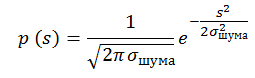
The probability that a pixel contains a signal s is equal to p (s). An example of a sequence filled with normally distributed noise with a variance of 1 and a mean of 0:

There is also a signal with a constant signal-to-noise ratio, SNR = E_signal / σ_shum = const. We have the right to write this when the signal size is approximately equal to the pixel size. Our signal is also set by Gaussian:
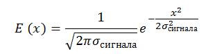
For simplicity, we assume that σ_signal = 0.25 L, where L is the pixel size. And this means that for a signal located in the center of a pixel a pixel will contain the signal energy from - 2σ to + 2σ:
This is how the previous sequence with noise will look, on top of which a signal with SNR = 5 superimposed with center 4.1 is superimposed:

By the way, do you know how to generate a normal distribution ?
It's funny, but many use the central limit theorem for its generation. In this method, 6 linearly distributed values are added in the range of -0.5 to 0.5. It is believed that the value obtained is distributed normally with a variance equal to one. But this method gives incorrect distribution tails, with large deviations. If we take exactly 6 values, then max = | min | = 3 = 3 * σ. Which immediately cuts off 0.2% of implementations. When generating an image of 100 * 100, such events should occur in 20 pixels, which is not so little.
There are good algorithms: Box-Muller Transform, George Marsalya Transform
On Habré there is a good article on this topic.
All these methods are based on converting the linear distribution on the interval [0; 1] to the normal distribution in a mathematical way.
Much has been written about neural networks. I will try not to go into details, having limited to only links and main points.
The neural network consists of neurons. Nobody knows how a neuron works in humans, but there are many beautiful models. On Habré there were many interesting articles about neurons: 1 , 2 , etc.
In the problem I took the simplest scheme of neurons as a basis, when a sequence of signals is fed to the input of the neuron, which is summed and run through the activation function:
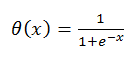
Where is the activation function:
What does such a neuron do in such a model and why does it need the activation function?
A neuron makes a comparison with a certain pattern for which it learns. And the activation function is a trigger that makes a decision about how the pattern coincided and normalizes the decision. For some reason, it often seems to me that a neuron is like a transistor, but this is a lyrical digression:

Why not do the step activation function? There are many reasons, but the main thing about which will be described a little lower is a learning feature, which requires differentiation of the neuron function. The above activation function has a very good differential:

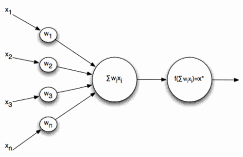
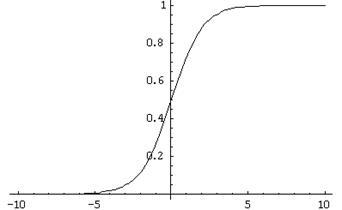
We have a network. How to solve a problem? The classic way to solve a simple problem is to create a neural network of the following type:
It has an input signal, one hidden layer (where each neuron is connected to all input elements) and an output neuron. Training such a network is essentially the setting of all the coefficients w and v.
We'll do it almost like this, but by optimizing for a puzzle. Why train each neuron of the hidden layer for each pixel of the input image? The maximum signal takes three pixels, and most likely even two. Therefore, we connect each neuron of the hidden layer with only three adjacent pixels:
With this configuration, the neuron is trained on the neighborhood of the image, starting to work as a local detector. The array of learning elements for the hidden layer (1..N) will look like:
As an experiment, I introduced two output neurons, but it didn’t make much sense, as it turned out later.
Neural networks of this type are among the oldest used in the works. Recently, more and more people use convolutional networks. About convolutional networks have repeatedly written on Habré: 1 , 2 .
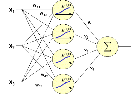
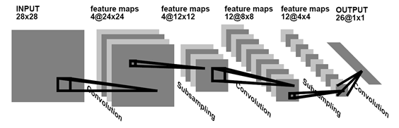
A convolution network is a network that searches for and remembers existing patterns that are universal for the entire image. Usually, to demonstrate what a neural network is, draw such an image:
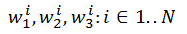
But when you start trying to code it, the brain enters into a stupor from “how can this be applied to reality”. But in reality, the above example of a neural network is transferred to a convolutional network with just one action. To do this, it’s enough to learn that the elements w 1 1 , ..., w 1 N are not different elements, but the same element w 1 . Then, as a result of learning the hidden layer, only three elements w 1 , w 2 , w 3 will be found, representing a convolution.
However, as it turned out, one convolution is not enough for solving the problem, you need to enter the second one, but this is simply done by increasing the number of elements in the hidden layer to 1..2N, while elements 1..N teach the first convolution, and elements N. 2N - the second.
A neural network is simple to draw, but not so easy to train. When you do it for the first time, the brain turns a little. But, fortunately, in RuNet there are two very good articles, after which everything becomes clear as day: 1 , 2
The first one illustrates the logic and the order of training very well, the second is a well-written mathematical essence: where does it come from the formulas, how is the neural network initialized, how to read and apply coefficients correctly.
In general, the method of back propagation of an error is as follows: send a known signal to the input, extend it to the output neurons, compare it with the required result. If there is a mismatch, then the magnitude of the error is multiplied by the weight of the connection and transmitted to all neurons in the last layer. When all the neurons know their mistake, then shift their learning coefficients so that the error decreases.
If anything, then you should not be afraid of learning. For example, the definition of an error is done in one line like this:
And weights correction like this:
To begin with, as promised, we will consider "what should be." Let us have the SNR (signal / noise) ratio = 3. In this case, the signal is 3 times higher than the noise variance. Let's draw the probability that the signal in a pixel takes the value X:
The graph immediately displays graphs only for the probability distribution of noise and a graph of the probability distribution of the signal + noise at a point with the ratio SNR = 3. In order to make a decision about finding a signal, you need to select a certain Xs, all values more than it should be considered a signal, all values less - noise. Let us draw the probability that we made a decision on a false alarm and on the omission of an object (for the red graph, this is its integral, for the blue “1-integral”):
The intersection point for such graphs is usually called EER (Equal Error Rate). At this point, the probability of a wrong decision is equal to the probability of losing the object.
In this problem we have 10 input signals. How to choose an EER point for such a situation? Simple enough. The probability that a false alarm does not occur at the selected value of Xs will be equal (integral over the blue graph from the first figure):
Accordingly, the probability that a false alarm does not occur in 10 pixels is equal to:
The probability that at least 1 false alarm has occurred is 1-P. Let's draw the 1-P graph and, next to it, the graph of the probability of missing an object (let's duplicate from the second graph):
So the EER point for the signal and noise at SNR = 3 is in the region of two and in it EER≈0.2. And what will give the neural network?
It can be seen that the neural network will be slightly worse than the problem solved on the fingers. But it is not all that bad. In the mathematical consideration, we did not take into account several features (for example, the signal may not fall in the center of the pixel). Without going too deep, you can say that it does not greatly worsen the statistics, but it still worsens.
To be honest, I was encouraged by this result. The network copes well with a purely mathematical task.
Nevertheless, my main task was to create a neural network from scratch and poke it with a wand. In this section there will be a couple of funny gifs about network behavior. The network turned out far from ideal (I think that the article will be accompanied by devastating comments from professionals, because this topic is popular on Habré), but I learned a lot of design and writing features as a result of writing and now I’ll try not to repeat, so personally I am satisfied.
The first gif is for a regular network. The top bar is an input signal in time. SNR = 10, clearly visible signal. The lower two strips are the input to the summation of the last neuron. It is seen that the network has stabilized the image and when the signal is turned on and off, only the contrast of the inputs of the last neuron changes. It's funny that in the absence of a signal, the image is almost stationary.
The second gif is the same for the convolutional network. The number of inputs to the last neuron is increased by 2 times. But in principle, the structure does not change.
All the sources are here - github.com/ZlodeiBaal/NeuronNetwork . Written in C #. OpenCV has large ones, so after downloading you need to unpack inside the lib.rar folder. Either download the project immediately, do not need to unpack anything - yadi.sk/d/lZn2ZJ_BWc4DB .
The code was written for 2 pm somewhere, so far from industrial standards, but it seems to be understandable (I wrote the article on Habr longer, I must admit).
Sitting in the evening and suffering from the fact that you need to do something useful, but do not want to, I came across another article on neural networks and caught fire. It is necessary to finally do your neural network. The idea is trivial: everyone loves neural networks, there are plenty of open source examples. I sometimes had to use LeNet and networks from OpenCV. But I was always alarmed that I knew their characteristics and mechanics only from pieces of paper. And between the knowledge of "neural networks are trained by the method of reverse propagation" and understanding how to do this lies a huge gap. And then I decided. It's time to sit and do everything with your own hands for 1-2 evenings, to understand and understand.
A neural network without a task that a horse without a rider. To solve a neural network made on the knee a serious task - to spend a lot of time for debugging and processing. Therefore, a simple task was needed. One of the simplest tasks in signal processing that can be solved purely mathematically is the problem of detecting white noise. The advantage of the problem is that it can be solved on a piece of paper; one can estimate the accuracy of the resulting network in comparison with a mathematical solution. Indeed, it is not in every task that one can assess how well a neural network has worked out simply by checking with the formula.
')
Problem
First, we formulate the problem. Suppose we have a sequence of N elements. Each sequence element has noise, with zero expectation and unit variance. There is a signal E, which can be in this sequence with the center from 0.5 to N-0.5. The signal will be set by Gaussian with such a dispersion that, when located in the center of the pixel, most of the energy will be in the same pixel (it will be boring with quite a point). It is necessary to decide whether there is a signal in the sequence or not.
“What a synthetic challenge!” You say. But it is not so. Such a task arises every time you work with point objects. It can be stars in an image, it can be a reflected radio (sound, optical) pulse in a time sequence, it can even be some microorganisms under a microscope, not to mention airplanes and satellites in a telescope.
We write a little more strictly. Let there is a sequence of signals l 0 ... I n , containing normal noise with constant dispersion and zero expectation:
The probability that a pixel contains a signal s is equal to p (s). An example of a sequence filled with normally distributed noise with a variance of 1 and a mean of 0:
There is also a signal with a constant signal-to-noise ratio, SNR = E_signal / σ_shum = const. We have the right to write this when the signal size is approximately equal to the pixel size. Our signal is also set by Gaussian:
For simplicity, we assume that σ_signal = 0.25 L, where L is the pixel size. And this means that for a signal located in the center of a pixel a pixel will contain the signal energy from - 2σ to + 2σ:
This is how the previous sequence with noise will look, on top of which a signal with SNR = 5 superimposed with center 4.1 is superimposed:
By the way, do you know how to generate a normal distribution ?
It's funny, but many use the central limit theorem for its generation. In this method, 6 linearly distributed values are added in the range of -0.5 to 0.5. It is believed that the value obtained is distributed normally with a variance equal to one. But this method gives incorrect distribution tails, with large deviations. If we take exactly 6 values, then max = | min | = 3 = 3 * σ. Which immediately cuts off 0.2% of implementations. When generating an image of 100 * 100, such events should occur in 20 pixels, which is not so little.
There are good algorithms: Box-Muller Transform, George Marsalya Transform
On Habré there is a good article on this topic.
All these methods are based on converting the linear distribution on the interval [0; 1] to the normal distribution in a mathematical way.
Neuron
Much has been written about neural networks. I will try not to go into details, having limited to only links and main points.
The neural network consists of neurons. Nobody knows how a neuron works in humans, but there are many beautiful models. On Habré there were many interesting articles about neurons: 1 , 2 , etc.
In the problem I took the simplest scheme of neurons as a basis, when a sequence of signals is fed to the input of the neuron, which is summed and run through the activation function:
Where is the activation function:
What does such a neuron do in such a model and why does it need the activation function?
A neuron makes a comparison with a certain pattern for which it learns. And the activation function is a trigger that makes a decision about how the pattern coincided and normalizes the decision. For some reason, it often seems to me that a neuron is like a transistor, but this is a lyrical digression:
Why not do the step activation function? There are many reasons, but the main thing about which will be described a little lower is a learning feature, which requires differentiation of the neuron function. The above activation function has a very good differential:
Neural network
We have a network. How to solve a problem? The classic way to solve a simple problem is to create a neural network of the following type:
It has an input signal, one hidden layer (where each neuron is connected to all input elements) and an output neuron. Training such a network is essentially the setting of all the coefficients w and v.
We'll do it almost like this, but by optimizing for a puzzle. Why train each neuron of the hidden layer for each pixel of the input image? The maximum signal takes three pixels, and most likely even two. Therefore, we connect each neuron of the hidden layer with only three adjacent pixels:
With this configuration, the neuron is trained on the neighborhood of the image, starting to work as a local detector. The array of learning elements for the hidden layer (1..N) will look like:
As an experiment, I introduced two output neurons, but it didn’t make much sense, as it turned out later.
Neural networks of this type are among the oldest used in the works. Recently, more and more people use convolutional networks. About convolutional networks have repeatedly written on Habré: 1 , 2 .
A convolution network is a network that searches for and remembers existing patterns that are universal for the entire image. Usually, to demonstrate what a neural network is, draw such an image:
But when you start trying to code it, the brain enters into a stupor from “how can this be applied to reality”. But in reality, the above example of a neural network is transferred to a convolutional network with just one action. To do this, it’s enough to learn that the elements w 1 1 , ..., w 1 N are not different elements, but the same element w 1 . Then, as a result of learning the hidden layer, only three elements w 1 , w 2 , w 3 will be found, representing a convolution.
However, as it turned out, one convolution is not enough for solving the problem, you need to enter the second one, but this is simply done by increasing the number of elements in the hidden layer to 1..2N, while elements 1..N teach the first convolution, and elements N. 2N - the second.
Training
A neural network is simple to draw, but not so easy to train. When you do it for the first time, the brain turns a little. But, fortunately, in RuNet there are two very good articles, after which everything becomes clear as day: 1 , 2
The first one illustrates the logic and the order of training very well, the second is a well-written mathematical essence: where does it come from the formulas, how is the neural network initialized, how to read and apply coefficients correctly.
In general, the method of back propagation of an error is as follows: send a known signal to the input, extend it to the output neurons, compare it with the required result. If there is a mismatch, then the magnitude of the error is multiplied by the weight of the connection and transmitted to all neurons in the last layer. When all the neurons know their mistake, then shift their learning coefficients so that the error decreases.
If anything, then you should not be afraid of learning. For example, the definition of an error is done in one line like this:
public void ThetaForNode(Neuron t1, Neuron t2, int myname) { // BPThetta = t1.mass[myname] * t1.BPThetta + t2.mass[myname] * t2.BPThetta; } And weights correction like this:
public void CorrectWeight(double Speed, ref double[] massOut) { for (int i = 0; i < mass.Length; i++) { // + ****(1-) massOut[i] = massOut[i] + Speed * BPThetta * input[i] * RESULT * (1 - RESULT); } } Result
To begin with, as promised, we will consider "what should be." Let us have the SNR (signal / noise) ratio = 3. In this case, the signal is 3 times higher than the noise variance. Let's draw the probability that the signal in a pixel takes the value X:
The graph immediately displays graphs only for the probability distribution of noise and a graph of the probability distribution of the signal + noise at a point with the ratio SNR = 3. In order to make a decision about finding a signal, you need to select a certain Xs, all values more than it should be considered a signal, all values less - noise. Let us draw the probability that we made a decision on a false alarm and on the omission of an object (for the red graph, this is its integral, for the blue “1-integral”):
The intersection point for such graphs is usually called EER (Equal Error Rate). At this point, the probability of a wrong decision is equal to the probability of losing the object.
In this problem we have 10 input signals. How to choose an EER point for such a situation? Simple enough. The probability that a false alarm does not occur at the selected value of Xs will be equal (integral over the blue graph from the first figure):
Accordingly, the probability that a false alarm does not occur in 10 pixels is equal to:
The probability that at least 1 false alarm has occurred is 1-P. Let's draw the 1-P graph and, next to it, the graph of the probability of missing an object (let's duplicate from the second graph):
So the EER point for the signal and noise at SNR = 3 is in the region of two and in it EER≈0.2. And what will give the neural network?
It can be seen that the neural network will be slightly worse than the problem solved on the fingers. But it is not all that bad. In the mathematical consideration, we did not take into account several features (for example, the signal may not fall in the center of the pixel). Without going too deep, you can say that it does not greatly worsen the statistics, but it still worsens.
To be honest, I was encouraged by this result. The network copes well with a purely mathematical task.
Annex 1
Nevertheless, my main task was to create a neural network from scratch and poke it with a wand. In this section there will be a couple of funny gifs about network behavior. The network turned out far from ideal (I think that the article will be accompanied by devastating comments from professionals, because this topic is popular on Habré), but I learned a lot of design and writing features as a result of writing and now I’ll try not to repeat, so personally I am satisfied.
The first gif is for a regular network. The top bar is an input signal in time. SNR = 10, clearly visible signal. The lower two strips are the input to the summation of the last neuron. It is seen that the network has stabilized the image and when the signal is turned on and off, only the contrast of the inputs of the last neuron changes. It's funny that in the absence of a signal, the image is almost stationary.
The second gif is the same for the convolutional network. The number of inputs to the last neuron is increased by 2 times. But in principle, the structure does not change.
Appendix 2
All the sources are here - github.com/ZlodeiBaal/NeuronNetwork . Written in C #. OpenCV has large ones, so after downloading you need to unpack inside the lib.rar folder. Either download the project immediately, do not need to unpack anything - yadi.sk/d/lZn2ZJ_BWc4DB .
The code was written for 2 pm somewhere, so far from industrial standards, but it seems to be understandable (I wrote the article on Habr longer, I must admit).
Source: https://habr.com/ru/post/229851/
All Articles