Graphic models in machine learning. Yandex Workshop
Despite the enormous popularity of the apparatus of graphic models for solving the problem of structural classification, the task of adjusting their parameters in a training sample has long remained open. In his report, Dmitry Vetrov , spoke about the generalization of the support vector method and some features of its application for setting parameters of graphic models. Dmitry is the head of the Bayesian methods group, an associate professor at the CMC of Moscow State University and a teacher at the SAD.
Video report.
Report outline:
')
The very concept of machine learning is quite simple - it is, if we speak figuratively, the search for relationships in the data. The data is presented in the classical formulation by a set of objects taken from the same general population, each object has observed variables, there are hidden variables. Observed variables (we will refer to them as X ) are often called signs, respectively, hidden variables ( T ) are those to be defined. In order to establish this relationship between observables and hidden variables, it is assumed that we have a training set, i.e. a set of objects for which both observable and hidden components are known. Looking at it, we are trying to set up some decisive rules that will allow us later on, when we see a set of signs, to evaluate the hidden components. The training procedure looks approximately as follows: a set of admissible decision rules are fixed, which are usually set using weights ( W ), and then in some way during the training these weights are adjusted. Immediately, inevitably, the problem of retraining arises, if we have a too rich family of admissible decision rules, then in the learning process we can easily go to the case when we predict its hidden component perfectly well for the training sample, but the forecast for new objects is bad. Researchers in the field of machine learning have spent many years and efforts to remove this problem from the agenda. At the present time, it seems that somehow it has succeeded.
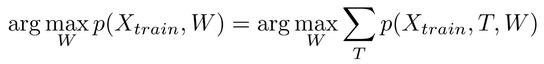
The Bayesian paradigm is a subsection of machine learning, and in this case it is assumed that the relationship between tunable parameters W , observable variables X and hidden variables T is modeled as some joint distribution, for example, into all three groups of variables. Accordingly, in the classical formulation of machine learning problems, i.e., when it is assumed that the data is a collection of objects taken from the same general population of independent objects, this joint distribution can be represented in this relatively simple form:

The first multiplier is responsible for the distribution of the hidden variable with known signs and a given decision rule. The second factor is responsible for the distribution of the observed variables for a given decision rule (the so-called discriminative models). This factor does not interest us, since we do not model the distribution of observable variables. But more generally, the so-called generative models, it has a place to be. And finally, the last factor, which inevitably follows, if we simply consider the rule for working with probabilities, this is the prior distribution on the weights W , that is, on the values of the parameters of the decision rule. And it is precisely the fact that we have the opportunity to set this prior distribution, which was probably the key reason why the Bayesian methods have been booming over the last 10 years. For a long time, until the mid-nineties, the Bayesian approach to the theory of probability was rather skeptically perceived by researchers for the reason that it assumes that we somehow have to specify a prior distribution on the parameters. And the traditional question was - where to get it. The likelihood function, of course, is determined by the data, and the prior distribution is taken from the ceiling? It is clear that if we take the a priori distribution in different ways, we will end up with different results, applying the Bayes formula. Therefore, for a long time, the Bayesian approach seemed like a mind game. Nevertheless, around the mid-nineties, a flurry of work began, proving that the general, standard methods of machine learning can be significantly improved if we take into account the specifics of the problem being solved.
It turned out that there are a lot of specifics where there is, it seems like all tasks are reduced to standard statements, but in most cases there is some specificity, some a priori preferences for one or another form of the decision rule. Those. in fact, preferences for certain values of weights W. And then the question arose, how can this be combined with the quality of work of the decision rule on the training set? Traditionally, the machine learning procedure looks like minimization of a training error, i.e. we are trying to build a decision rule in order to predict as accurately as possible the variables T for the training sample for which they are known. Those. we can evaluate the quality. This is one indicator. Another indicator is that we consider some values of W to be preferable.
How can all this be linked in single terms? It turned out that this is possible in the framework of the Bayes paradigm. Qualitative in training is characterized by a likelihood function, which is a probabilistic sense, and preference for parameters is characterized by an a priori distribution. Accordingly, the likelihood function and a priori distribution are perfectly combined within the framework of the Bayes formula and lead to a posteriori distributions on the values of the parameters W , which we tune during the training. Thus, the Bayesian paradigm made it possible to correctly, in common terms, combine both the accuracy of the training set and our a priori preferences for weights, which in quite a lot of applied problems arose quite organically, and, accordingly, the introduction of these a priori preferences made it possible to significantly improve the quality of the decision rules obtained . In addition, since the end of the nineties and in the zero years, more advanced means have appeared, which allow also a priori distribution to parametrize in a certain cunning way and adjust according to the data. Those. I pressed the button, and the prior distribution most appropriate for the task was automatically tuned, after which the machine learning procedure went.
These methods are already well developed. It would not be a great exaggeration to say that the classical formulation of the machine learning problem is solved. And as often happens in life, as soon as we closed the classical production, it immediately turned out that we were more interested in non-classical productions, which turned out to be much richer and more interesting. Non-classical formulation in this case is a situation when hidden variables of objects are interdependent. Those. we cannot determine the hidden variable of each object by looking only at the signs of this object, as was assumed in the traditional machine learning problem. Moreover, it depends not only and not so much on the attributes of other objects, but on the hidden variables of other objects. Accordingly, we cannot determine the hidden variable of each object independently, only in aggregate. Below I will give a large number of examples of tasks with interrelated hidden components. You can see that these relationships, i.e. awareness of the fact that the hidden variables in our sample are interdependent, opens up tremendous opportunities for additional regularization of problems. Those. ultimately to further improve the accuracy of the solution.

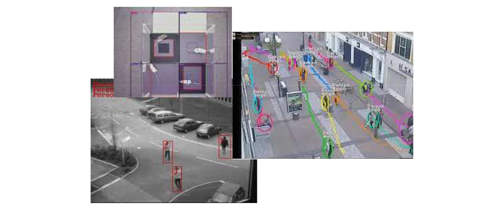
The first most classic example is image segmentation. This is a tool that solves such problems with interdependent hidden variables, and the boom of graphical models actually began with it. The task has become extremely popular with the development of digital cameras. What it is? For each pixel we are trying to put some class mark. In the simplest case with binary segmentation, we are trying to separate the object from the background. In more complex cases, we are trying to introduce some semantics for objects as well. In principle, this task can be considered as a standard classification problem. Each pixel is an object, each pixel can belong to one of the K classes, each pixel has a specific set of features. In the simplest case, it is a color, you can remove textural signs, some contextual information, but it seems quite obvious that in this case we have some specificity. Neighboring pixels most likely belong to the same class, simply because in the segmentation task we assume that we will have some compact areas as a result of the segmentation. As soon as we try to formalize this fact, it inevitably follows that we cannot classify or segment each pixel in isolation from the rest, we can only segment the entire image at once. Here is the simplest task in which interdependencies between hidden variables appeared.
The next task is video tracking. We can process each frame independently, say, search or identify pedestrians, identify pedestrians. Or do tracking of mice. The mice on top look very similar, you need to track them so that each mouse can still be identified correctly. Attempts to put colored strokes on wool are harshly suppressed by biologists who claim that the mouse will then be under stress. Accordingly, the mice are all the same, it is necessary at each moment to know where our mouse is, in order to analyze their behavior. It is clear that we are not able to solve the problem on a separate frame. We need to take into account neighboring frames, preferably in large quantities. We again have interdependencies between hidden variables, where the mouse identifier acts as a hidden variable.

The analysis of social networks now is quite an obvious task. Each user of social networks, of course, can be analyzed independently of the others, but it is obvious that at the same time we will lose a significant amount of information. For example, we are trying to analyze users for their opposition to the current regime. If I have a “Navalny for presidency!” Or “Navalny for mayors!” Banner, I, of course, can be identified as an oppositionist, but if I am more careful about this and do not post such banners, then I’ll define that I sympathize with the opposition, You can only analyze my less cautious friends, which these banners happily hang. If it turns out that I, with a large number of such people, am in the status of friends, then the probability that I myself also sympathize with these trends rises somewhat. Well, if you get away from such a similar topic, then, say, the same task of targeted advertising can be solved much better if we use not only data about a specific user (say, personal data that he reported on his page), but also looking at his circle of friends.
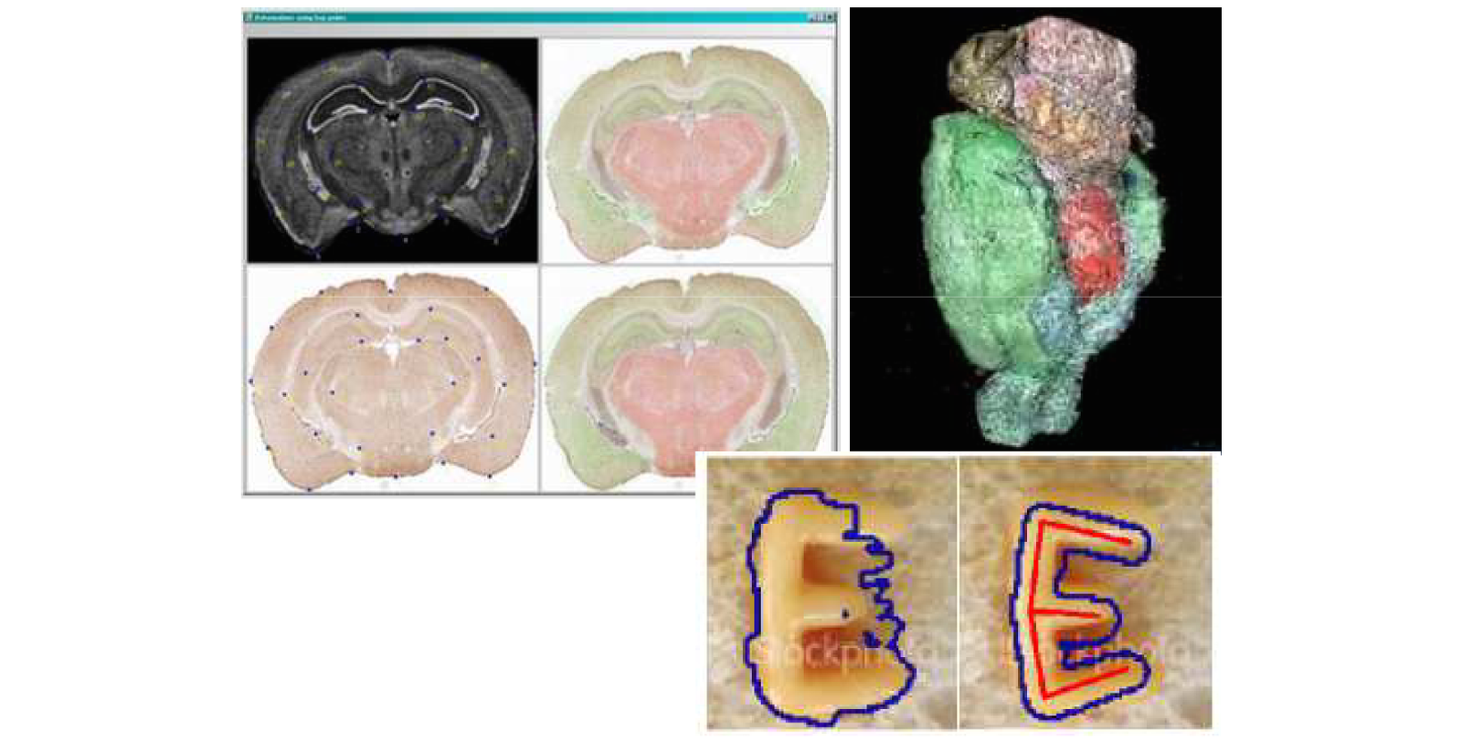
The next task is to register images for building three-dimensional models from an image, inscribing an image into a two- or three-dimensional model. This task assumes that the images undergo some deformation during registration. Of course, we can try to look for the deformation for each pixel independently of the others, but it is clear that in this case we will not get any elastic deformation, the result will be rather pitiable. Although formally we will enter each pixel somewhere, and the error for each pixel will be minimal. At the same time, the entire image will simply crumble if every pixel is deformed independently. As one of the ways to account for these interdependencies, you can use the apparatus of graphical models, which allows you to analyze the interdependencies of hidden variables.
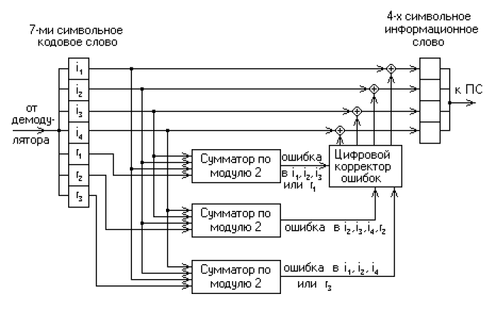
There is another important task. It is not often mentioned about it, but in fact it is very relevant and, most likely, in the coming years, relevance will only increase. This is the decoding of noisy messages. Now we are surrounded by mobile devices. Data transfer with their help is not very reliable, the channels are terribly overloaded. Obviously, the need for traffic exceeds the current capabilities, so naturally the problem arises of drawing up such a protocol, which on the one hand would be noise-resistant, and on the other hand, would have high throughput. Here we are faced with a curious phenomenon. Since the fifties of the last century, when the theory of information was developed by Claude Shannon, it is known that for each communication channel there is a certain limiting throughput for a given interference intensity.
A theoretical formula was derived. More information than Shannon’s theorem predicts cannot be transmitted over a noisy channel in principle. But it turns out that as we approach this theoretical limit, i.e. the more effectively we try to transmit information using some tricky archiving schemes and adding control bits, which are just aimed at correcting errors, the more difficult we are to decode this message. Those. The most effective noise-resistant codes are extremely difficult to decode. There are no simple decoding formulas. Accordingly, if we reach the Shannon limit, the decoding complexity increases exponentially. We can encode and transmit the message, but are no longer able to decrypt it. It turned out that modern codes developed and standardized in the zero years (they are now used in most mobile devices) are close to this theoretically possible limit, and their decoding uses the so-called message transfer algorithm based on the trust propagation algorithm that appeared in theory of graphical models, which arose in an attempt to solve a problem with interrelated hidden variables.
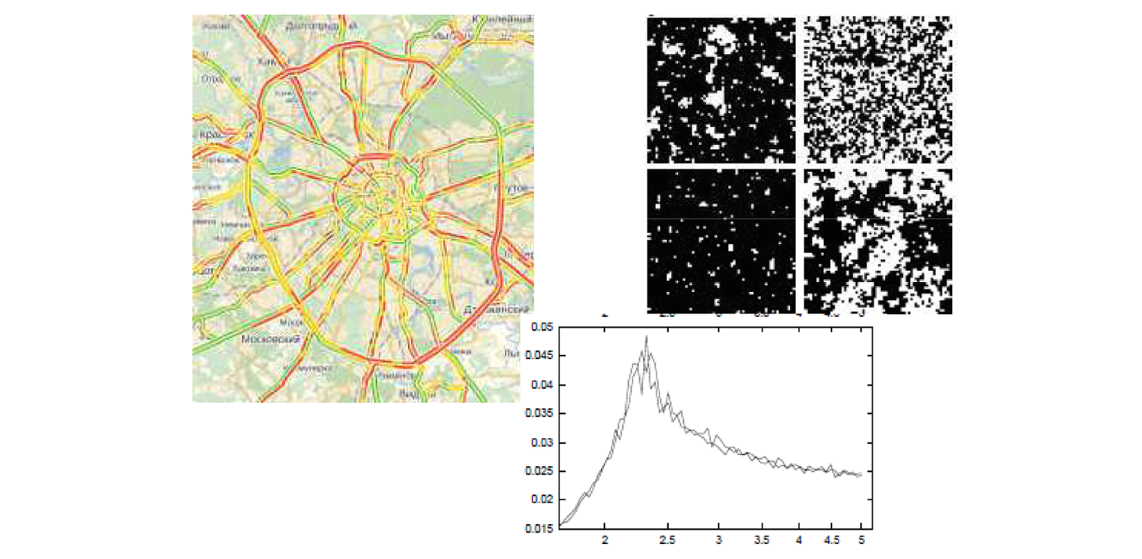
In the late nineties, a task that I conditionally called simulation modeling or modeling of agent environments also became popular. This is an attempt to analyze the behavior of systems consisting of a large number of interacting agents. The task is extremely interesting, there are no strict methods for its solution. Therefore, most of these problems are solved using the Monte Carlo simulation method in various modifications. A simple example is traffic simulation. Vehicles act as an agent, it is clear that we cannot model the behavior of cars out of context, since all drivers make decisions looking at their closest neighbors on the highway. And it turned out that the introduction of even the simplest interaction between motorists into the model made it possible to get an amazing result. First, it was established first in theory and then in practice that there is some critical limit for the intensity of the flow. If the flow exceeds this limit, it becomes metastable, i.e. unstable. The slightest deviation from the norm (for example, one of the drivers braked a little more sharply and immediately drove on) leads to the fact that traffic jams immediately grow tens of kilometers. This means that when the transport channel is overloaded, it can still function without traffic jams, but a traffic jam can occur almost on level ground.
First we got it in theory, then we were convinced that in practice it really happens. Indeed, for each route, depending on its interchanges, there is a certain maximum throughput at which the stream is still moving steadily. This effect of a jump-like transition from a stable movement to a dead congestion is one example of phase transitions. It turned out that in agent systems such phenomena are very often encountered, and the conditions under which a phase transition takes place are not at all trivial. In order to be able to model, the necessary funds are needed. If I already say that these are multi-agent systems, then agents are objects, and objects interact with each other. We have interdependencies between variables describing each agent.
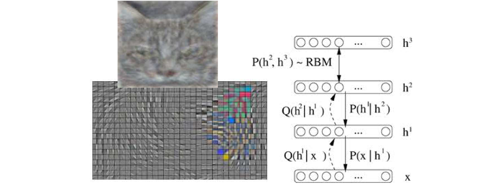
The next example is deep learning. The picture is taken from the report of a representative of Google Corporation at the ICML 2012 conference, where they made a splash with the fact that they were able to significantly improve the quality of classifications of photos from the Flickr database by applying a relatively young paradigm in machine learning - deep learning. In some form, this is the reincarnation of neural networks in a new way. Traditional neural networks have successfully ordered to live long. Nevertheless, they inspired in some form the emergence of a different approach. Depth networks, Boltzmann networks, which from themselves represent a certain set of limited Boltzmann machines. In essence, these are layers of interconnected binary variables. These variables can be interpreted as hidden variables that, when making a decision, are somehow tuned to the observed variables. But the peculiarity is that all hidden variables here are interdependent in a cunning manner. To train such a network and in order to make a decision within such a network, we again have to apply methods based on the analysis of objects with interdependent variables.

Finally, the last application that came to my mind was a collaborative filtering or recommender system. Also a relatively new direction. However, for obvious reasons, it is gaining increasing popularity. Now online stores are actively developing, providing tens and hundreds of thousands of items, i.e. such an amount that no user can even grasp. It is clear that the user will view only those products that he previously somehow selected from this gigantic range. Accordingly, there are tasks to build a recommendation system. You can build it by analyzing not only a specific user (which products he already bought, his personal data, gender, age), but also the behavior of other users who bought similar products. Again, interdependencies arise between variables.
I hope that I was able to show the relevance of the fact that you really have to move away from the classical machine learning productions, and that the world is actually more complicated and interesting. We have to go to the tasks when we have objects that have interdependent hidden components. As a result, it is necessary to model a strongly multidimensional distribution, for example, on hidden components. Here comes the trouble. Imagine the simplest situation. Say, a thousand objects, each of them has a hidden variable binary, can take the values 0/1. If we want to specify a joint distribution, where everything depends on everything, it means that we need to formally define a thousandth distribution on binary variables. The question is: how many parameters will we need for this in order to specify this distribution? Answer: 2 1000 or about 10 300 . For comparison, the number of atoms in the observable universe is 10 80 . Obviously, we cannot set 10,300 , even if we combine the computing power of the whole world. Imagine a 30x30 image in which each pixel can take on an object / background value. We cannot calculate the distribution on the set of such pictures in principle, since the distribution is discrete and requires 2,1000 parameters.
What to do? The first option that comes to mind is, suppose that each pixel is distributed independently of the others. Then we need only a thousand parameters, i.e. the probability that each pixel takes a value of, say, 1. Then -1 is the probability that it has assumed the value 0. This is how standard machine learning works. One small problem - all variables have become independent. Therefore, we cannot solve any of the listed problems in this way. The question is: how will we restrict ourselves to a small number of parameters, but to define a distribution, in which everything depends on everything? And it is here that the paradigm of graphic models comes to the rescue, which assumes that in our case the joint distribution can be represented as a product of a certain number of factors defined on overlapping subsets of variables. In order to set these factors, we traditionally used an undirected graph that links some objects in the sample to each other, and the factorization system is determined by the maximum clicks of this graph.
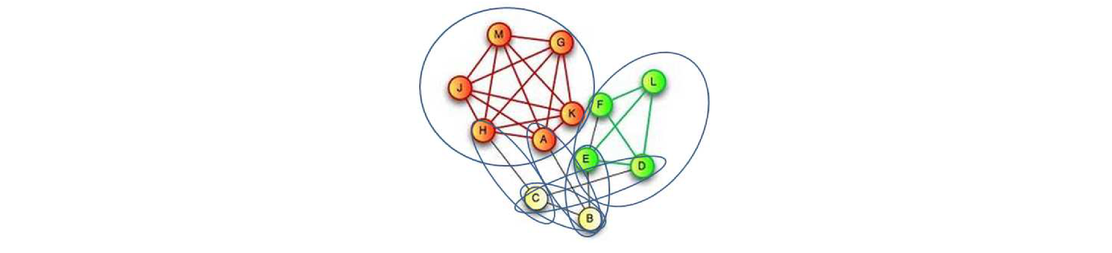
These clicks are very small, the maximum clicks are size 2. This means that we only need three parameters to specify the distribution for clicks of size 2. Each such factor can be defined by a small number of variables, and, as a result, since there are not too many such factors. , we can describe the joint distribution with a relatively small number of parameters. On the other hand, even a relatively simple factorization system gives us a guaranteed situation when all of our variables depend on all. Those. we obtained complete interdependence by limiting ourselves to some factorization system. The factorization system defines conditional independence.
What, within the framework of the theory of graphical models, are the main tasks? The apparatus was proposed in the late nineties: a joint distribution of the model in the form of some factorization system. Suppose we have introduced such a system. Then we come back to the problems of machine learning, which in the Bayesian formulation assumed that we assigned a distribution to three groups of values: hidden variables T , observed variables X, and the parameter of the decision rule W. It turned out that within the framework of graphical models the tasks are very similar.
The rest of the report is devoted to the analysis of the task of training with the teacher. View the full report here .
Video report.
Report outline:
- Bayesian methods in machine learning.
- Tasks with interdependent hidden variables.
- Probabilistic Graphic Models
- Support vector machine and its generalization for setting parameters of graphic models.
')
The very concept of machine learning is quite simple - it is, if we speak figuratively, the search for relationships in the data. The data is presented in the classical formulation by a set of objects taken from the same general population, each object has observed variables, there are hidden variables. Observed variables (we will refer to them as X ) are often called signs, respectively, hidden variables ( T ) are those to be defined. In order to establish this relationship between observables and hidden variables, it is assumed that we have a training set, i.e. a set of objects for which both observable and hidden components are known. Looking at it, we are trying to set up some decisive rules that will allow us later on, when we see a set of signs, to evaluate the hidden components. The training procedure looks approximately as follows: a set of admissible decision rules are fixed, which are usually set using weights ( W ), and then in some way during the training these weights are adjusted. Immediately, inevitably, the problem of retraining arises, if we have a too rich family of admissible decision rules, then in the learning process we can easily go to the case when we predict its hidden component perfectly well for the training sample, but the forecast for new objects is bad. Researchers in the field of machine learning have spent many years and efforts to remove this problem from the agenda. At the present time, it seems that somehow it has succeeded.
The Bayesian paradigm is a subsection of machine learning, and in this case it is assumed that the relationship between tunable parameters W , observable variables X and hidden variables T is modeled as some joint distribution, for example, into all three groups of variables. Accordingly, in the classical formulation of machine learning problems, i.e., when it is assumed that the data is a collection of objects taken from the same general population of independent objects, this joint distribution can be represented in this relatively simple form:
The first multiplier is responsible for the distribution of the hidden variable with known signs and a given decision rule. The second factor is responsible for the distribution of the observed variables for a given decision rule (the so-called discriminative models). This factor does not interest us, since we do not model the distribution of observable variables. But more generally, the so-called generative models, it has a place to be. And finally, the last factor, which inevitably follows, if we simply consider the rule for working with probabilities, this is the prior distribution on the weights W , that is, on the values of the parameters of the decision rule. And it is precisely the fact that we have the opportunity to set this prior distribution, which was probably the key reason why the Bayesian methods have been booming over the last 10 years. For a long time, until the mid-nineties, the Bayesian approach to the theory of probability was rather skeptically perceived by researchers for the reason that it assumes that we somehow have to specify a prior distribution on the parameters. And the traditional question was - where to get it. The likelihood function, of course, is determined by the data, and the prior distribution is taken from the ceiling? It is clear that if we take the a priori distribution in different ways, we will end up with different results, applying the Bayes formula. Therefore, for a long time, the Bayesian approach seemed like a mind game. Nevertheless, around the mid-nineties, a flurry of work began, proving that the general, standard methods of machine learning can be significantly improved if we take into account the specifics of the problem being solved.
It turned out that there are a lot of specifics where there is, it seems like all tasks are reduced to standard statements, but in most cases there is some specificity, some a priori preferences for one or another form of the decision rule. Those. in fact, preferences for certain values of weights W. And then the question arose, how can this be combined with the quality of work of the decision rule on the training set? Traditionally, the machine learning procedure looks like minimization of a training error, i.e. we are trying to build a decision rule in order to predict as accurately as possible the variables T for the training sample for which they are known. Those. we can evaluate the quality. This is one indicator. Another indicator is that we consider some values of W to be preferable.
How can all this be linked in single terms? It turned out that this is possible in the framework of the Bayes paradigm. Qualitative in training is characterized by a likelihood function, which is a probabilistic sense, and preference for parameters is characterized by an a priori distribution. Accordingly, the likelihood function and a priori distribution are perfectly combined within the framework of the Bayes formula and lead to a posteriori distributions on the values of the parameters W , which we tune during the training. Thus, the Bayesian paradigm made it possible to correctly, in common terms, combine both the accuracy of the training set and our a priori preferences for weights, which in quite a lot of applied problems arose quite organically, and, accordingly, the introduction of these a priori preferences made it possible to significantly improve the quality of the decision rules obtained . In addition, since the end of the nineties and in the zero years, more advanced means have appeared, which allow also a priori distribution to parametrize in a certain cunning way and adjust according to the data. Those. I pressed the button, and the prior distribution most appropriate for the task was automatically tuned, after which the machine learning procedure went.
These methods are already well developed. It would not be a great exaggeration to say that the classical formulation of the machine learning problem is solved. And as often happens in life, as soon as we closed the classical production, it immediately turned out that we were more interested in non-classical productions, which turned out to be much richer and more interesting. Non-classical formulation in this case is a situation when hidden variables of objects are interdependent. Those. we cannot determine the hidden variable of each object by looking only at the signs of this object, as was assumed in the traditional machine learning problem. Moreover, it depends not only and not so much on the attributes of other objects, but on the hidden variables of other objects. Accordingly, we cannot determine the hidden variable of each object independently, only in aggregate. Below I will give a large number of examples of tasks with interrelated hidden components. You can see that these relationships, i.e. awareness of the fact that the hidden variables in our sample are interdependent, opens up tremendous opportunities for additional regularization of problems. Those. ultimately to further improve the accuracy of the solution.
Image segmentation
The first most classic example is image segmentation. This is a tool that solves such problems with interdependent hidden variables, and the boom of graphical models actually began with it. The task has become extremely popular with the development of digital cameras. What it is? For each pixel we are trying to put some class mark. In the simplest case with binary segmentation, we are trying to separate the object from the background. In more complex cases, we are trying to introduce some semantics for objects as well. In principle, this task can be considered as a standard classification problem. Each pixel is an object, each pixel can belong to one of the K classes, each pixel has a specific set of features. In the simplest case, it is a color, you can remove textural signs, some contextual information, but it seems quite obvious that in this case we have some specificity. Neighboring pixels most likely belong to the same class, simply because in the segmentation task we assume that we will have some compact areas as a result of the segmentation. As soon as we try to formalize this fact, it inevitably follows that we cannot classify or segment each pixel in isolation from the rest, we can only segment the entire image at once. Here is the simplest task in which interdependencies between hidden variables appeared.
Video tracking
The next task is video tracking. We can process each frame independently, say, search or identify pedestrians, identify pedestrians. Or do tracking of mice. The mice on top look very similar, you need to track them so that each mouse can still be identified correctly. Attempts to put colored strokes on wool are harshly suppressed by biologists who claim that the mouse will then be under stress. Accordingly, the mice are all the same, it is necessary at each moment to know where our mouse is, in order to analyze their behavior. It is clear that we are not able to solve the problem on a separate frame. We need to take into account neighboring frames, preferably in large quantities. We again have interdependencies between hidden variables, where the mouse identifier acts as a hidden variable.
Social Network Analysis
The analysis of social networks now is quite an obvious task. Each user of social networks, of course, can be analyzed independently of the others, but it is obvious that at the same time we will lose a significant amount of information. For example, we are trying to analyze users for their opposition to the current regime. If I have a “Navalny for presidency!” Or “Navalny for mayors!” Banner, I, of course, can be identified as an oppositionist, but if I am more careful about this and do not post such banners, then I’ll define that I sympathize with the opposition, You can only analyze my less cautious friends, which these banners happily hang. If it turns out that I, with a large number of such people, am in the status of friends, then the probability that I myself also sympathize with these trends rises somewhat. Well, if you get away from such a similar topic, then, say, the same task of targeted advertising can be solved much better if we use not only data about a specific user (say, personal data that he reported on his page), but also looking at his circle of friends.
Fill 2D and 3D models
The next task is to register images for building three-dimensional models from an image, inscribing an image into a two- or three-dimensional model. This task assumes that the images undergo some deformation during registration. Of course, we can try to look for the deformation for each pixel independently of the others, but it is clear that in this case we will not get any elastic deformation, the result will be rather pitiable. Although formally we will enter each pixel somewhere, and the error for each pixel will be minimal. At the same time, the entire image will simply crumble if every pixel is deformed independently. As one of the ways to account for these interdependencies, you can use the apparatus of graphical models, which allows you to analyze the interdependencies of hidden variables.
Decoding Noisy Messages
There is another important task. It is not often mentioned about it, but in fact it is very relevant and, most likely, in the coming years, relevance will only increase. This is the decoding of noisy messages. Now we are surrounded by mobile devices. Data transfer with their help is not very reliable, the channels are terribly overloaded. Obviously, the need for traffic exceeds the current capabilities, so naturally the problem arises of drawing up such a protocol, which on the one hand would be noise-resistant, and on the other hand, would have high throughput. Here we are faced with a curious phenomenon. Since the fifties of the last century, when the theory of information was developed by Claude Shannon, it is known that for each communication channel there is a certain limiting throughput for a given interference intensity.
A theoretical formula was derived. More information than Shannon’s theorem predicts cannot be transmitted over a noisy channel in principle. But it turns out that as we approach this theoretical limit, i.e. the more effectively we try to transmit information using some tricky archiving schemes and adding control bits, which are just aimed at correcting errors, the more difficult we are to decode this message. Those. The most effective noise-resistant codes are extremely difficult to decode. There are no simple decoding formulas. Accordingly, if we reach the Shannon limit, the decoding complexity increases exponentially. We can encode and transmit the message, but are no longer able to decrypt it. It turned out that modern codes developed and standardized in the zero years (they are now used in most mobile devices) are close to this theoretically possible limit, and their decoding uses the so-called message transfer algorithm based on the trust propagation algorithm that appeared in theory of graphical models, which arose in an attempt to solve a problem with interrelated hidden variables.
Simulation
In the late nineties, a task that I conditionally called simulation modeling or modeling of agent environments also became popular. This is an attempt to analyze the behavior of systems consisting of a large number of interacting agents. The task is extremely interesting, there are no strict methods for its solution. Therefore, most of these problems are solved using the Monte Carlo simulation method in various modifications. A simple example is traffic simulation. Vehicles act as an agent, it is clear that we cannot model the behavior of cars out of context, since all drivers make decisions looking at their closest neighbors on the highway. And it turned out that the introduction of even the simplest interaction between motorists into the model made it possible to get an amazing result. First, it was established first in theory and then in practice that there is some critical limit for the intensity of the flow. If the flow exceeds this limit, it becomes metastable, i.e. unstable. The slightest deviation from the norm (for example, one of the drivers braked a little more sharply and immediately drove on) leads to the fact that traffic jams immediately grow tens of kilometers. This means that when the transport channel is overloaded, it can still function without traffic jams, but a traffic jam can occur almost on level ground.
First we got it in theory, then we were convinced that in practice it really happens. Indeed, for each route, depending on its interchanges, there is a certain maximum throughput at which the stream is still moving steadily. This effect of a jump-like transition from a stable movement to a dead congestion is one example of phase transitions. It turned out that in agent systems such phenomena are very often encountered, and the conditions under which a phase transition takes place are not at all trivial. In order to be able to model, the necessary funds are needed. If I already say that these are multi-agent systems, then agents are objects, and objects interact with each other. We have interdependencies between variables describing each agent.
Deep learning
The next example is deep learning. The picture is taken from the report of a representative of Google Corporation at the ICML 2012 conference, where they made a splash with the fact that they were able to significantly improve the quality of classifications of photos from the Flickr database by applying a relatively young paradigm in machine learning - deep learning. In some form, this is the reincarnation of neural networks in a new way. Traditional neural networks have successfully ordered to live long. Nevertheless, they inspired in some form the emergence of a different approach. Depth networks, Boltzmann networks, which from themselves represent a certain set of limited Boltzmann machines. In essence, these are layers of interconnected binary variables. These variables can be interpreted as hidden variables that, when making a decision, are somehow tuned to the observed variables. But the peculiarity is that all hidden variables here are interdependent in a cunning manner. To train such a network and in order to make a decision within such a network, we again have to apply methods based on the analysis of objects with interdependent variables.
Collaborative filtering
Finally, the last application that came to my mind was a collaborative filtering or recommender system. Also a relatively new direction. However, for obvious reasons, it is gaining increasing popularity. Now online stores are actively developing, providing tens and hundreds of thousands of items, i.e. such an amount that no user can even grasp. It is clear that the user will view only those products that he previously somehow selected from this gigantic range. Accordingly, there are tasks to build a recommendation system. You can build it by analyzing not only a specific user (which products he already bought, his personal data, gender, age), but also the behavior of other users who bought similar products. Again, interdependencies arise between variables.
Graphic models
I hope that I was able to show the relevance of the fact that you really have to move away from the classical machine learning productions, and that the world is actually more complicated and interesting. We have to go to the tasks when we have objects that have interdependent hidden components. As a result, it is necessary to model a strongly multidimensional distribution, for example, on hidden components. Here comes the trouble. Imagine the simplest situation. Say, a thousand objects, each of them has a hidden variable binary, can take the values 0/1. If we want to specify a joint distribution, where everything depends on everything, it means that we need to formally define a thousandth distribution on binary variables. The question is: how many parameters will we need for this in order to specify this distribution? Answer: 2 1000 or about 10 300 . For comparison, the number of atoms in the observable universe is 10 80 . Obviously, we cannot set 10,300 , even if we combine the computing power of the whole world. Imagine a 30x30 image in which each pixel can take on an object / background value. We cannot calculate the distribution on the set of such pictures in principle, since the distribution is discrete and requires 2,1000 parameters.
What to do? The first option that comes to mind is, suppose that each pixel is distributed independently of the others. Then we need only a thousand parameters, i.e. the probability that each pixel takes a value of, say, 1. Then -1 is the probability that it has assumed the value 0. This is how standard machine learning works. One small problem - all variables have become independent. Therefore, we cannot solve any of the listed problems in this way. The question is: how will we restrict ourselves to a small number of parameters, but to define a distribution, in which everything depends on everything? And it is here that the paradigm of graphic models comes to the rescue, which assumes that in our case the joint distribution can be represented as a product of a certain number of factors defined on overlapping subsets of variables. In order to set these factors, we traditionally used an undirected graph that links some objects in the sample to each other, and the factorization system is determined by the maximum clicks of this graph.
These clicks are very small, the maximum clicks are size 2. This means that we only need three parameters to specify the distribution for clicks of size 2. Each such factor can be defined by a small number of variables, and, as a result, since there are not too many such factors. , we can describe the joint distribution with a relatively small number of parameters. On the other hand, even a relatively simple factorization system gives us a guaranteed situation when all of our variables depend on all. Those. we obtained complete interdependence by limiting ourselves to some factorization system. The factorization system defines conditional independence.
Main tasks
What, within the framework of the theory of graphical models, are the main tasks? The apparatus was proposed in the late nineties: a joint distribution of the model in the form of some factorization system. Suppose we have introduced such a system. Then we come back to the problems of machine learning, which in the Bayesian formulation assumed that we assigned a distribution to three groups of values: hidden variables T , observed variables X, and the parameter of the decision rule W. It turned out that within the framework of graphical models the tasks are very similar.
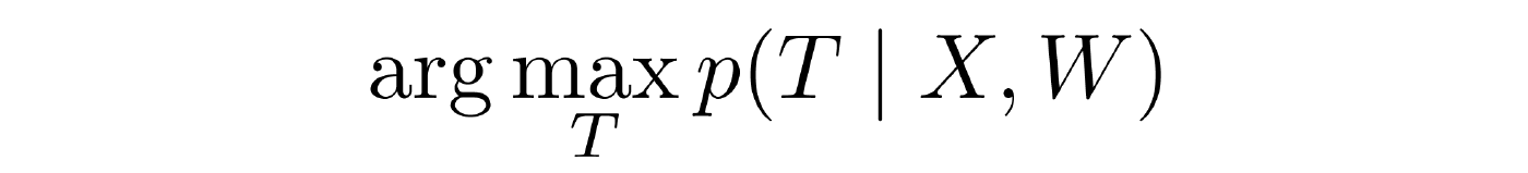
- Decision-making. The decision rule W is set , there is a sample in which we see observable variables. The task is to evaluate the hidden variables. As applied to standard machine learning tasks, the problem is solved easily and is not even considered by anyone. In graphic models, the problem has already become essentially non-trivial and far from always solvable.
- Definition of the normalization constant Z. Calculate it is not always easy.
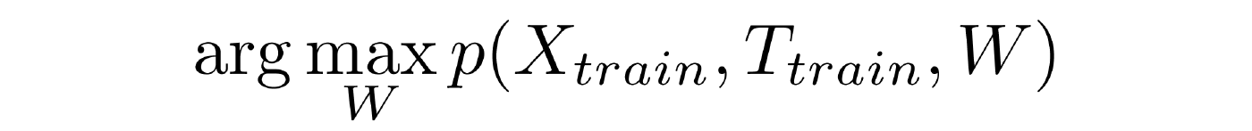
- Training with a teacher . Given the training sample, in which we know not only the observed variables, but also hidden ones. This is a set of interrelated objects. It is required to find the vector W , which converts the joint distribution to a maximum.
- Teaching without a teacher. Given a sample, but in it we only know the observable components, the hidden ones we do not know. We want to set up our decision rule. The task turns out to be extremely difficult, because there are quite a lot of T configurations.
- Marginal distribution . Given a sample, the observable components of X are known, the decision rule W is known, but we want to find not the most likely configuration of all the hidden variables of the sample, but the distribution into hidden variables for a single object. The task is often relevant in applications. Solved nontrivially.

The rest of the report is devoted to the analysis of the task of training with the teacher. View the full report here .
Source: https://habr.com/ru/post/229555/
All Articles