How to make binary classifier work a little bit better

Disclaimer: A post is written based on this . I suspect that most readers are well aware of how the Naive Bayes classifier works, so I propose only a glimpse of what it says before going under the cat.

Problem solving using machine learning algorithms has long been firmly established in our lives. This happened for all understandable and objective reasons: cheaper, simpler, faster than explicitly coding the algorithm for solving each individual problem. Usually, the “black boxes” of classifiers (it is unlikely that the same VC will offer you its corpus of marked names), which does not allow them to be fully managed.
Here I would like to talk about how to try to achieve the “best” results of the binary classifier, what characteristics the binary classifier has, how to measure them, and how to determine that the result of the work has become “better”.

Theory. Short course

1. Binary classification

Let be - many objects - finite set of classes. Categorize object - use mapping . When , such a classification is called binary , because we have only 2 options at the output. For simplicity, we will further assume that , because absolutely any problem of binary classification can lead to this. Usually , the result of mapping an object into a class is a real number, and if it is above a given threshold , then the object is classified as positive , and its class is 1.

2. Table of contingency binary classifier

Obviously, the predicted class of the object obtained by mapping can either match in a real class or not. Total 4 options in the amount. This is very clearly demonstrated by this tablet:

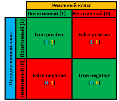
If we know the quantitative values ​​of each of the assessments - we know all that is possible about this classifier and can dig further.
(I deliberately do not use the terms of the type "error of the first kind" because it seems to me not obvious and unnecessary)
We will continue to use the following notation:

• - the number of True Positive results for this sample.
• - the number of True Negative results for this sample.
• - False Positive number of results for this sample.
• - the number of False Negative results for this sample.

3. Characteristics of a binary classifier

Accuracy (precision) - shows how many of the predicted positive objects turned out to be really positive.

Fullness (recall) - shows how much of the total number of real positive objects, it was predicted as a positive class.

These two characteristics are essential for any binary classifier. Which of the characteristics is more important - it all depends on the task. For example, if we want to create a “school search engine,” then it will be in our interest to remove “non-childish” content from the issue, and here completeness is much more important than accuracy. In the case of determining the gender of the name - we are more interested in accuracy than completeness.
F-measure (F-measure) - a characteristic that allows you to give an estimate at the same time for accuracy and completeness.

Coefficient sets the balance of precision and completeness. When The F-measure gives equal weight to both characteristics. This F-measure is called balanced, or

False Positive Rate ( ) - shows how many of the total number of real negative objects turned out to be incorrectly predicted.

4. ROC curve and its AUC

ROC curve - a graph that allows you to assess the quality of the binary classification. The graph shows the dependence of TPR (completeness) on FPR with varying threshold. At the point (0,0), the threshold is minimal, and TPR and FPR are also minimal. An ideal case for a classifier is the passage of a graph through a point (0,1). Obviously, the graph of this function is always monotonically non-decreasing.

AUC (Area Under Curve) - this term (the area under the graph) gives a quantitative characteristic of the ROC curve: the more the better. AUC is equivalent to the probability that the classifier will assign a greater value to a randomly selected positive object than to a randomly chosen negative object. That is why it was previously said that, as a rule , the positive class is rated higher than the negative.
When AUC = 0.5 , then this classifier is equal to random. If AUC <0.5 , then you can simply flip the values ​​produced by the classifier.
')

Cross validation

There are many methods of cross validation (assessing the quality of a binary classifier), and this is a topic for a separate article. Here I just want to consider one of the most popular methods in order to understand how this thing works at all, and why it is needed.
Of course, it is possible to build a ROC curve for any sample. However, the ROC curve constructed from the training set will be shifted left-up due to retraining. To avoid this and get the most objective assessment, cross-validation is used.
K-fold cross validation - the pool is split into k folds, then each fold is used for the test, while the remaining k-1 folds are used for training. The value of the parameter k can be arbitrary. In this case, I used it to be 10. For the given gender classifier of the name, the following AUC results were obtained (get_features_simple is one significant letter, get_features_complex is 3 significant letters)

fold	get_features_simple	get_features_complex
0	0.978011	0.962733
one	0.96791	0.944097
2	0.963462	0.966129
3	0.966339	0.948452
four	0.946586	0.945479
five	0.949849	0.989648
6	0.959984	0.943266
7	0.979036	0.958863
eight	0.986469	0.951975
9	0.962057	0.980921
avg	0.9659703	0.9591563

Practice

1. Preparation

The entire repository is here .
I took the same tagged file and replaced it with “m” for 1, “f” - 0. We’ll use this pool for training, like the author of the previous article. Armed with the first page of issuing a favorite search engine and awk, I rivet the list of names that are not in the original. This pool will be used for the test.
Changed the classification function so that it returns the probabilities of positive and negative classes, and not logarithmic indicators.

2. Implementation and use

As written in the title, my task was to make the binary classifier work better than it works by default. In this case, we want to learn how to determine the gender of a name, better than the probability of Naive Bayes 0.5. For this, this simplest utility was written. It is written in C ++, because gcc is everywhere. The implementation itself is nothing interesting, it seems to me. With a key -? or --help you can read the help, I tried to describe it in as much detail as possible.
And now, in fact, what we were going to: the assessment of the classifier and its tuning. At the output, nbc.py creates a sheet from the files with the results of the classification, I use them directly below. For our purposes, we will clearly see the graphs of accuracy from the threshold, completeness from the threshold and F-measure from the threshold. They can be built as follows:

 $ ./OptimalThresholdFinder -A 3 -P 1 < names_test_pool.txt_simple -x thr -y prc -p plot_test_thr_prc_simple.txt $ ./OptimalThresholdFinder -A 3 -P 1 < names_test_pool.txt_simple -x thr -y tpr -p plot_test_thr_tpr_simple.txt $ ./OptimalThresholdFinder -A 3 -P 1 < names_test_pool.txt_simple -x thr -y fms -p plot_test_thr_fms_simple.txt $ ./OptimalThresholdFinder -A 3 -P 1 < names_test_pool.txt_simple -x thr -y fms -p plot_test_thr_fms_0.7_simple.txt -a 0.7 

For educational purposes, I made 2 F-measures from the threshold, with different weights. The second weight was chosen 0.7, because in our problem we are more interested in accuracy than completeness. The default graph is based on 10,000 different points, which is a lot for such simple data, but these are uninteresting optimization subtleties. In the same way, by constructing graph data for get_features_complex, we obtain the following results:


From the graphs it becomes obvious that the classifier shows the best results by no means at the threshold of 0.5. The graph of the F-measure clearly demonstrates that the "complex feature" gives the best result on all the variation of the threshold. This is quite logical, given that it is also "complicated." We obtain the threshold values ​​at which the F-measure reaches a maximum:

 $ ./OptimalThresholdFinder -A 3 -P 1 < names_test_pool.txt_simple --target fms --argument thr --argval 0 Optimal threshold = 0.8 Target function = 0.911937 Argument = 0.8 $ ./OptimalThresholdFinder -A 3 -P 1 < names_test_pool.txt_complex --target fms --argument thr --argval 0 Optimal threshold = 0.716068 Target function = 0.908738 Argument = 0.716068 

Agree, these values ​​are much better than those that turned out to be at the threshold of 0.5.

Conclusion

With such simple manipulations, we were able to choose the optimal Naive Bayes threshold to determine the gender of the name that works better than the default threshold. This raises a reasonable question, how do we determine that it works “better”? I have repeatedly mentioned that accuracy is more important to us in this task than completeness, but the question of how important it is is very, very difficult, so a balanced F-measure was used to evaluate the classifier’s performance, which in this case can be an objective indicator quality.
What is much more interesting, the results of the binary classifier based on the “simple” and “complex” features turned out to be approximately the same, differing in the value of the optimal threshold.