Fur rendering using Shells and Fins algorithm

Hi, Habr! My today's post on programming graphics will not be as voluminous as the previous ones. In almost any difficult business, there is sometimes a place for frivolous, and today we will render the seals. More precisely, I want to talk about the implementation of the algorithm rendering fur Shells and Fins (SAF) traditionally for Direct3D 11 and OpenGL 4. For details, I ask under the cat.

The SAF fur rendering algorithm, as the name implies, consists of 2 parts: the rendering of shells and the rendering of fins. Perhaps some of these names seem funny, but they fully reflect what is created by the algorithm to create the illusion of a fleecy surface. More details on the implementation of the algorithm for Direct3D 10 can be found in the article and the NVidia demo, my demo for Direct3D 11 and OpenGL 4 can be found here . The project is called Demo_Fur. You will need Visual Studio 2012/2013 and CMake to build.

Shells and Fins algorithm

The fur consists of a huge number of hairs, to draw each of them separately at the current moment is not possible in real time, although NVidia had certain attempts . In order to create the illusion of a fleecy surface, a technology is applied, somewhat resembling voxel rendering. A three-dimensional texture is prepared, which is a small area of ​​the fur surface. Each voxel in it determines the likelihood of villi passing through itself, which, from a graphical point of view, determines the value of transparency at a particular point during rendering. Such a three-dimensional texture can be generated (one of the methods described here ). A natural question arises how to render this texture. For this, “shells” are drawn around the geometry, i.e. copies of the original geometry, formed by scaling this geometry to small values. It turns out a kind of matryoshka, on each layer of which is superimposed a layer of three-dimensional texture of fur. Layers are drawn in series with alpha blending turned on, which results in some illusion of fleecy. However, this is not enough for the material to resemble fur. To achieve the goal, you must select the correct lighting model.
Fur belongs to the category of pronounced anisotropic materials. Classical lighting models (for example, the Blinna-Phong model) treat surfaces as isotropic, i.e. surface properties do not depend on its orientation. In practice, this means that when the plane is rotated around its normal, the nature of the illumination does not change. Illumination models of this class for calculating the shadows use the angle between the normal and the direction of light incidence. Anisotropic lighting models use tangents (vectors perpendicular to the normals, which together with the normals and binormals form the basis) to calculate the illumination. Read more about anisotropic lighting here .
Anisotropic illumination is calculated separately for each fur layer. The values ​​of the tangent at one or another point on the surface are determined using a tangent map. The tangent map is formed in much the same way as the well-known normal map . In the case of fur texture, the tangent vector will be the normalized direction of the hair. Thus, the three-dimensional texture of the fur will contain 4 channels. A packed tangent vector will be stored in RGB, the alpha channel will contain the probability of passing the villus through this point. Add to this an account of the self-shadowing of the fur and get quite realistic looking material.
The illusion will be broken if the person carefully looks at the outer edges of the object. At certain angles between the faces in a situation where one face is visible and the other is not, fur layers may be invisible to the observer. In order to avoid this situation, additional geometry is formed on such edges, which is drawn along their normals. The result is somewhat similar to the fins of the fish, which determined the second part of the algorithm name.

Implementation on Direct3D 11 and OpenGL 4

The implementations on both APIs are generally identical, only minor details differ. Rendering will be done according to the following scheme:

1. Rendering the uncovered parts of the scene. In my demo for such parts the standard lighting model Blinna-Phong is used.
2. Rendering fins. We will implement geometry extrusion using a geometry shader. To understand whether it is necessary to draw an edge between two polygons, it is necessary to determine whether this edge is external to the object. A sign of this will be the values ​​of the angles between the normals to the polygons and the normalized vector of vision. If these values ​​have a different sign, then the edge will be external, and therefore it must be pulled out. Geometric shaders in Direct3D and OpenGL can work with a limited number of primitives. We need to simultaneously process 2 adjacent polygons with one common edge. To represent this structure, 4 vertices are minimally needed, which is graphically shown in the figure below on the left.
   
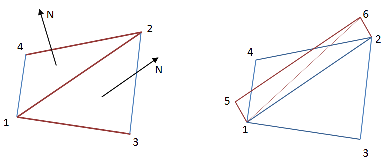
   The right side of the figure shows the extrusion of a common edge 1-2 and the formation of two new polygons 1-5-6 and 1-6-2.
   The primitive that consists of 4 vertices is D3D_PRIMITIVE_TOPOLOGY_LINELIST_ADJ (GL_LINES_ADJACENCY in OpenGL). In order to use it, we need to prepare a special index buffer. It is rather simple to build such a buffer if there are data on the contiguity of triangles in the 3D model. The index buffer will contain groups of 4 indices describing 2 adjacent triangles.
   It is important to note here that it is not possible to easily obtain adjacency data for any model. For most smoothed models, this is not a problem, however, at the edges of the smoothing groups, vertices are usually duplicated to achieve proper lighting. This means the actual lack of adjacency in the index buffer in the presence of visual adjacency. In this case, it is necessary to look for adjacent triangles, guided not only by indices, but also by the actual location of the vertices in space. This task is no longer so trivial, since in this case as many triangles can divide into one face.
   Geometric shaders for pulling "fins" are listed below under the spoilers.
   ')
   
   HLSL Geometry Shader for Direct3D 11

   #include <common.h.hlsl> struct GS_INPUT { float4 position : SV_POSITION; float2 uv0 : TEXCOORD0; float3 normal : TEXCOORD1; }; struct GS_OUTPUT { float4 position : SV_POSITION; float3 uv0 : TEXCOORD0; }; texture2D furLengthMap : register(t0); SamplerState defaultSampler : register(s0); [maxvertexcount(6)] void main(lineadj GS_INPUT pnt[4], inout TriangleStream<GS_OUTPUT> triStream) { float3 c1 = (pnt[0].position.xyz + pnt[1].position.xyz + pnt[2].position.xyz) / 3.0f; float3 c2 = (pnt[1].position.xyz + pnt[2].position.xyz + pnt[3].position.xyz) / 3.0f; float3 viewDirection1 = -normalize(viewPosition - c1); float3 viewDirection2 = -normalize(viewPosition - c2); float3 n1 = normalize(cross(pnt[0].position.xyz - pnt[1].position.xyz, pnt[2].position.xyz - pnt[1].position.xyz)); float3 n2 = normalize(cross(pnt[1].position.xyz - pnt[2].position.xyz, pnt[3].position.xyz - pnt[2].position.xyz)); float edge = dot(n1, viewDirection1) * dot(n2, viewDirection2); float furLen = furLengthMap.SampleLevel(defaultSampler, pnt[1].uv0, 0).r * FUR_LENGTH; if (edge > 0 && furLen > 1e-3) { GS_OUTPUT p[4]; p[0].position = mul(pnt[1].position, modelViewProjection); p[0].uv0 = float3(pnt[1].uv0, 0); p[1].position = mul(pnt[2].position, modelViewProjection); p[1].uv0 = float3(pnt[2].uv0, 0); p[2].position = mul(float4(pnt[1].position.xyz + pnt[1].normal * furLen, 1), modelViewProjection); p[2].uv0 = float3(pnt[1].uv0, 1); p[3].position = mul(float4(pnt[2].position.xyz + pnt[2].normal * furLen, 1), modelViewProjection); p[3].uv0 = float3(pnt[2].uv0, 1); triStream.Append(p[2]); triStream.Append(p[1]); triStream.Append(p[0]); triStream.RestartStrip(); triStream.Append(p[1]); triStream.Append(p[2]); triStream.Append(p[3]); triStream.RestartStrip(); } } 

   
   
   GLSL Geometry Shader for OpenGL 4.3

    #version 430 core layout(lines_adjacency) in; layout(triangle_strip, max_vertices = 6) out; in VS_OUTPUT { vec2 uv0; vec3 normal; } gsinput[]; out vec3 texcoords; const float FUR_LAYERS = 16.0f; const float FUR_LENGTH = 0.03f; uniform mat4 modelViewProjectionMatrix; uniform sampler2D furLengthMap; uniform vec3 viewPosition; void main() { vec3 c1 = (gl_in[0].gl_Position.xyz + gl_in[1].gl_Position.xyz + gl_in[2].gl_Position.xyz) / 3.0f; vec3 c2 = (gl_in[1].gl_Position.xyz + gl_in[2].gl_Position.xyz + gl_in[3].gl_Position.xyz) / 3.0f; vec3 viewDirection1 = -normalize(viewPosition - c1); vec3 viewDirection2 = -normalize(viewPosition - c2); vec3 n1 = normalize(cross(gl_in[0].gl_Position.xyz - gl_in[1].gl_Position.xyz, gl_in[2].gl_Position.xyz - gl_in[1].gl_Position.xyz)); vec3 n2 = normalize(cross(gl_in[1].gl_Position.xyz - gl_in[2].gl_Position.xyz, gl_in[3].gl_Position.xyz - gl_in[2].gl_Position.xyz)); float edge = dot(n1, viewDirection1) * dot(n2, viewDirection2); float furLen = texture(furLengthMap, gsinput[1].uv0).r * FUR_LENGTH; vec4 p[4]; vec3 uv[4]; if (edge > 0 && furLen > 1e-3) { p[0] = modelViewProjectionMatrix * vec4(gl_in[1].gl_Position.xyz, 1); uv[0] = vec3(gsinput[1].uv0, 0); p[1] = modelViewProjectionMatrix * vec4(gl_in[2].gl_Position.xyz, 1); uv[1] = vec3(gsinput[2].uv0, 0); p[2] = modelViewProjectionMatrix * vec4(gl_in[1].gl_Position.xyz + gsinput[1].normal * furLen, 1); uv[2] = vec3(gsinput[1].uv0, FUR_LAYERS - 1); p[3] = modelViewProjectionMatrix * vec4(gl_in[2].gl_Position.xyz + gsinput[2].normal * furLen, 1); uv[3] = vec3(gsinput[2].uv0, FUR_LAYERS - 1); gl_Position = p[2]; texcoords = uv[2]; EmitVertex(); gl_Position = p[1]; texcoords = uv[1]; EmitVertex(); gl_Position = p[0]; texcoords = uv[0]; EmitVertex(); EndPrimitive(); gl_Position = p[1]; texcoords = uv[1]; EmitVertex(); gl_Position = p[2]; texcoords = uv[2]; EmitVertex(); gl_Position = p[3]; texcoords = uv[3]; EmitVertex(); EndPrimitive(); } } 

   
   
   
3. Rendering "shells". Obviously, to obtain the proper number of layers of fur, the geometry must be drawn several times. For multiple drawing of geometry we will use hardware instansing. In order to determine which fur layer is drawn in the shader, it suffices to use the semantics of SV_InstanceID in Direct3D and the gl_InstanceID variable in OpenGL.
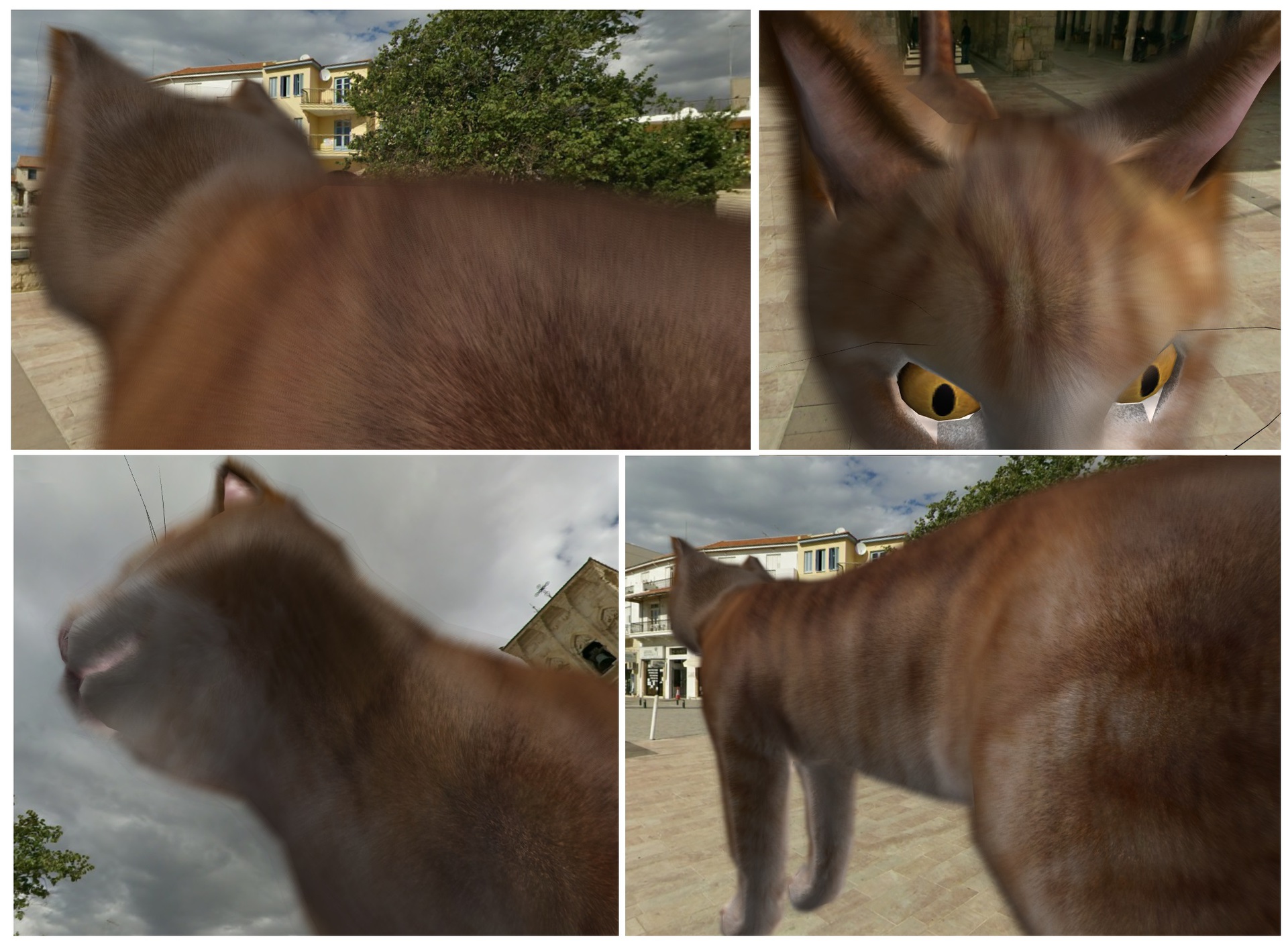
   To illuminate the fur, I used the Kajiya-Kay anisotropic model. An important detail was the use of a special texture to set the length of the fur. This texture is necessary to prevent the appearance of long fur in unexpected places (for example, around the cat's eyes). Pixel and fragment shaders for calculating the fur lighting are listed below under the spoilers.
   
   
   HLSL pixel shader for Direct3D 11

    #include <common.h.hlsl> struct PS_INPUT { float4 position : SV_POSITION; float3 uv0 : TEXCOORD0; float3 tangent : TEXCOORD1; float3 normal : TEXCOORD2; float3 worldPos : TEXCOORD3; }; texture2D diffuseMap : register(t1); texture3D furMap : register(t2); SamplerState defaultSampler : register(s0); float4 main(PS_INPUT input) : SV_TARGET { const float specPower = 30.0; float3 coords = input.uv0 * float3(FUR_SCALE, FUR_SCALE, 1.0f); float4 fur = furMap.Sample(defaultSampler, coords); clip(fur.a - 0.01); float4 outputColor = float4(0, 0, 0, 0); outputColor.a = fur.a * (1.0 - input.uv0.z); outputColor.rgb = diffuseMap.Sample(defaultSampler, input.uv0.xy).rgb; float3 viewDirection = normalize(input.worldPos - viewPosition); float3x3 ts = float3x3(input.tangent, cross(input.normal, input.tangent), input.normal); float3 tangentVector = normalize((fur.rgb - 0.5f) * 2.0f); tangentVector = normalize(mul(tangentVector, ts)); float TdotL = dot(tangentVector, light.direction); float TdotE = dot(tangentVector, viewDirection); float sinTL = sqrt(1 - TdotL * TdotL); float sinTE = sqrt(1 - TdotE * TdotE); outputColor.xyz = light.ambientColor * outputColor.rgb + light.diffuseColor * (1.0 - sinTL) * outputColor.rgb + light.specularColor * pow(abs((TdotL * TdotE + sinTL * sinTE)), specPower) * FUR_SPECULAR_POWER; float shadow = input.uv0.z * (1.0f - FUR_SELF_SHADOWING) + FUR_SELF_SHADOWING; outputColor.rgb *= shadow; return outputColor; } 

   
   
   GLSL Fragment Shader for OpenGL 4.3

    #version 430 core in VS_OUTPUT { vec3 uv0; vec3 normal; vec3 tangent; vec3 worldPos; } psinput; out vec4 outputColor; const float FUR_LAYERS = 16.0f; const float FUR_SELF_SHADOWING = 0.9f; const float FUR_SCALE = 50.0f; const float FUR_SPECULAR_POWER = 0.35f; // lights struct LightData { vec3 position; uint lightType; vec3 direction; float falloff; vec3 diffuseColor; float angle; vec3 ambientColor; uint dummy; vec3 specularColor; uint dummy2; }; layout(std430) buffer lightsDataBuffer { LightData lightsData[]; }; uniform sampler2D diffuseMap; uniform sampler2DArray furMap; uniform vec3 viewPosition; void main() { const float specPower = 30.0; vec3 coords = psinput.uv0 * vec3(FUR_SCALE, FUR_SCALE, 1.0); vec4 fur = texture(furMap, coords); if (fur.a < 0.01) discard; float d = psinput.uv0.z / FUR_LAYERS; outputColor = vec4(texture(diffuseMap, psinput.uv0.xy).rgb, fur.a * (1.0 - d)); vec3 viewDirection = normalize(psinput.worldPos - viewPosition); vec3 tangentVector = normalize((fur.rgb - 0.5) * 2.0); mat3 ts = mat3(psinput.tangent, cross(psinput.normal, psinput.tangent), psinput.normal); tangentVector = normalize(ts * tangentVector); float TdotL = dot(tangentVector, lightsData[0].direction); float TdotE = dot(tangentVector, viewDirection); float sinTL = sqrt(1 - TdotL * TdotL); float sinTE = sqrt(1 - TdotE * TdotE); outputColor.rgb = lightsData[0].ambientColor * outputColor.rgb + lightsData[0].diffuseColor * (1.0 - sinTL) * outputColor.rgb + lightsData[0].specularColor * pow(abs((TdotL * TdotE + sinTL * sinTE)), specPower) * FUR_SPECULAR_POWER; float shadow = d * (1.0 - FUR_SELF_SHADOWING) + FUR_SELF_SHADOWING; outputColor.rgb *= shadow; } 

As a result, we can get such seals.




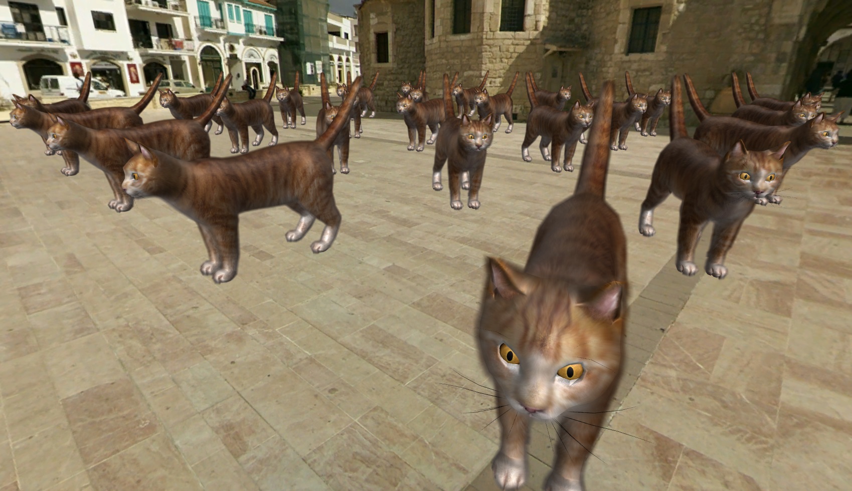
For comparison, the picture on the right shows the rendering of a cat using the Blinna-Phong model using normal maps.

Performance

The SAF algorithm is quite simple to implement, but it can significantly complicate the life of a video card. Each model will be drawn several times to obtain a specified number of layers of fur (I used 16 layers). In the case of complex geometry, this can be a significant performance drop. In the cat model used, the fur-covered part occupies approximately 3,000 polygons, therefore, about 48,000 polygons will be drawn for rendering the skin. When drawing "fins", the most simple geometric shader is not used, which can also affect the case of a highly detailed model.
Performance measurements were taken on a computer with the following configuration: AMD Phenom II X4 970 3.79GHz, 16Gb RAM, AMD Radeon HD 7700 Series, Windows 8.1.

Average frame time. 1920x1080 / MSAA 8x / full screen

API / Number of cats	one	25	100
Direct3d 11	2.73615ms	14.3022ms	42.8362ms
Opengl 4.3	2.5748ms	13.4807ms	34.2388ms

Overall, the implementation on OpenGL 4 roughly corresponds to the implementation on Direct3D 11 in terms of performance on an average and a small number of objects. On a large number of objects, implementation on OpenGL runs slightly faster.

Conclusion

The SAF algorithm is one of the few ways to implement fur in interactive rendering. However, it cannot be said that the algorithm is necessary to the overwhelming number of games. To date, a similar level of quality (and perhaps even higher) is achieved with the help of art and skilled hands of a graphic designer. The combination of translucent planes with well-chosen textures for representing hair and fur is the standard of modern games, and the considered algorithm and its variations are rather a matter of the games of the future.