Structure from Motion - classic implementation

There is such an interesting task - the construction of a 3D structure on a set of images (photos) - Structure from Motion. How can it be solved? After some thought, this algorithm comes to mind. We find the characteristic features (points) on all the images, compare them with each other and by triangulation we find their three-dimensional coordinates. There really is a problem - the camera position is unknown when shooting. Can you find them? It seems possible. Indeed, let us have N points on the frame and M frames. Then the unknowns will be 3 * N (three-dimensional coordinates of points) + 6 * (M - 1) (coordinates of cameras (instead of 6 there may be a different number, but this does not change the essence)). Equations we have 2 * M * N (each point on each image has two coordinates). It turns out that already for two images and 6 points the problem is solvable. Under the cut is a description of the conceptual scheme for solving the SfM problem (if possible without formulas - but with links for thoughtful study).

The plan is:

1. Find Key Points
2. Find matches between points for consecutive pairs of images (although it can be found for all pairs of images)
3. Filter false matches
4. Solve the system of equations and find the three-dimensional structure along with the camera positions

The plan seems to be simple and straightforward. And, of course, all the intrigue in the 3rd and 4th points.
')

1. Points

Finding points does not cause problems. There are lots of methods. The most famous is SIFT . He quite reliably finds the key points taking into account their scale and orientation (which is important when the camera moves arbitrarily). There are several open-source implementations of this method.

2. Compliance

Each point must be accompanied by its description (descriptor). If the descriptors of points on different images are close, then we can assume that the same physical object. The simplest descriptor is a small neighborhood of a point. But ideally, of course, the descriptor should be independent of the scale and orientation of the image. In the SIFT method it is used such. Then the search for matches is reduced to bypassing all the key points of one image and finding the closest descriptor on another image.

3. Filtering false matches.

It is clear that with any quality of the descriptor of false matches there will be many. They need to filter. Here we can distinguish two stages:

1. Geometry-independent filtering
2. Epipolar restriction filtering

Geometry-independent filtering is described in the same SIFT method. There are several simple filters, for example: the best fit from the first image to the second should match the best match from the second to the first.



Epipolar geometry. C and C ' are the optical centers of the cameras. If the point P in the first image is designed in m . Then, on the other image, its projection must be searched for on the straight line l ' _m .

The strongest filtering is, of course, using the epipolar constraint . Its geometric meaning is that for each point of one image its corresponding point on another image is on a certain line (which does not depend on the true three-dimensional coordinates of the point). Mathematically, this property is expressed by the equation m ^T Fm '= 0 . Here m = (u, v, 1) ^T are the homogeneous coordinates of the key point in the image, and F is the fundamental matrix. Most importantly, this ratio does not depend on the three-dimensional structure of the observed scene.

Since the fundamental matrix is ​​unknown to us, the following method can be used to filter out false matches:

1. Randomly select several points and calculate the fundamental matrix from them (the calculation method is described in [1], section 14.3.2).
2. Let us calculate how many more points satisfy the condition m ^T Fm '= 0 with a given accuracy.
3. If the number of points is large enough, stop the cycle, otherwise go to point 1.

This simple algorithm is called RANSAC and is ideal for our task. And yes - he is still quite cunning and you can suffer a lot with him too. Well, or you can use OpenCV .

4. Search for three-dimensional structure

It's time to finally figure out how the points in space are connected with the points on the image. Everything is simple - a projective transformation. Fortunately, the specifics of my task (observation in a telescope with a small field of view) made it possible to use the affine geometry of the camera. Geometric parameters of the camera consist of two parts:

• External parameters that determine the position of the camera in space (rotation matrix R 3x3 and shift vector t 3x1).
• Internal parameters that determine the design of the image on the CCD camera. These include scaling along each of the axes, the angle between the axes, and higher order distortion factors. For the case of square pixels and an affine camera, only one parameter remains - the scale k .

The observation equation (the relationship between the three-dimensional coordinates (X, Y, Z) ^{T of a} point and its position in the image (u, v) ^T ) can be written as:



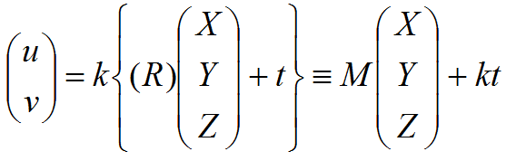
It is important to note here that the third row is ignored in affine geometry, and only two rows can be used from the rotation and shift matrices.

It turns out that we need to select the external (and internal) parameters of all the cameras and the three-dimensional coordinates of the points so that this relationship is performed as precisely as possible for all the points.

There are two ways to solve this problem. The first is to try to solve this non-linear system with a bunch of non-linear methods ( bundle adjustment ). The main problem here is obvious - it is necessary to be able to solve very large systems of nonlinear equations (or rather, to minimize the nonlinear function in a multidimensional space) and to achieve their convergence to the correct solution. Another way is to solve the problem analytically whenever possible. So we will do.

And here we are helped by the method of factorization. It turns out that using a singular decomposition one can solve the problem for an affine camera for the case when all points are visible from all cameras (in practice this means “for each pair of images separately”). A justification can be found in [1], section 18.2.

1. Shift all points on all images so that the center of mass is at the origin. This allows you to completely eliminate the shift vector from the equations.
2. We compose the observation matrix from the projection of all points found. . Then, having written all the matrixes of the cameras one under the other into the matrix M , and all three-dimensional points next to each other in the matrix X, we obtain the equation W = MX .
3. Find the singular decomposition W = UDV ^T. Then the camera matrices are obtained from the first three columns of U multiplied by singular values. The three-dimensional affine structure is obtained from the first three columns of the matrix V.

Too easy? Yes - there is a catch. The fact is that our solution was found up to an affine transformation, since we ignored the structure of the rotation matrix (and it is not arbitrary at all). To correct the situation, we must take into account that the cameras are described by orthogonal matrices, or simply noting that W = MX = MCC ^T X for any orthogonal matrix C (for a description of the method, see [2], section 12.4.2.)

The rotation matrix must satisfy the following conditions:


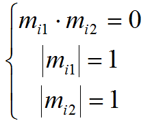
where m _ij - matrix lines of each camera. These restrictions can be used to search for a matrix C that reduces the affine structure to a Euclidean one:



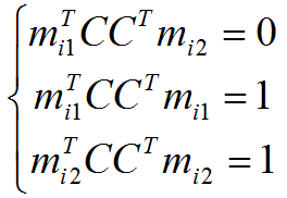
This system of equations is nonlinear with respect to C , but linear with D = CC ^T. From D, the matrix C is obtained by taking the square root of the matrix . Multiplying the matrixes of the cameras on the right by C , and the three-dimensional structure on the left by C ^T , we obtain the correct Euclidean structure, which also satisfies the observation matrix.

And finally - the union of three-dimensional structures from different pairs of cameras. There is a small nuance. The positions of the cameras obtained by us are centered relative to the set of points, and for different pairs of cameras the set of points is different. So you need to find on two pairs of cameras an intersecting set of points. Then, to recalculate the coordinates, you only need to find the transformation between these sets of points.
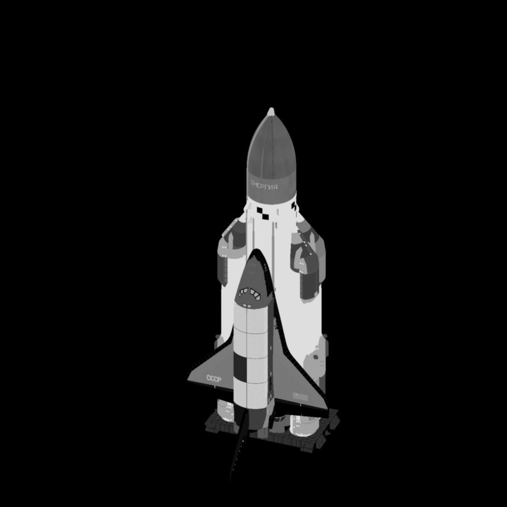
So we got a three-dimensional Euclidean (i.e. with preserving the angles and ratios of the lengths of segments) structure. In the image at the beginning of the post - this is the structure for the Energy-Buran model (one of the original images below). Such a structure is called sparse, because There are relatively few points. Getting out of this dense (dense) structure and stretching textures is another story.

Literature

1. R. Hartley, A. Zisserman, “Multiple View Geometry in Computer Vision”
2. Forsyth, Pons. “Computer vision. Modern approach "