On a compression algorithm for random signals (lossy)

annotation

It is known that there are various ways of generating pseudo-random numbers to simulate random variables on a computer. If we assume that a high-frequency (HF) signal is the implementation of a certain random variable, then there is a great temptation to choose a random variable model for this implementation that has known parameters for the implementation of its generation algorithm. Then we can represent the RF signal as this algorithm, and store only its parameters, i.e. compression occurs.

Description

Unfortunately, I do not know the methods that could restore the algorithm modeling it by implementing a random variable. The situation can be imagined as follows. Suppose we have a billiard table with one ball on it, we hit the ball with a cue on the ball and sample the position of the ball at regular intervals. We believe that there is no friction, and the blows against the walls of the table are absolutely elastic. So we get the implementation of a random variable by an algorithm similar to the congruent one. If we know the parameters of the table, the time after which the samples were taken, the position and velocity vector of the ball at any point in time, then we can restore the position of the ball at times and before and after the selected one. But if we only know the relative position of the ball on the plane and the fact that the samples were taken at regular intervals of time, we can only guess how the ball moved and where it will move. You can guess indefinitely. Having the implementation of the HF signal, we know the relative position of the ball at each of the sampling time points, but we need to build such a table and choose a time interval so that we take any sample (count) at the beginning and “hit” it with a cue, it takes all subsequent positions in the RF signal. It is intuitively clear that in the general case it is hardly possible to select such a table for the entire implementation.

Below, I will show you how to get around this problem and have a single billiard table (i.e., the parameters of the modeling algorithm) for working with different implementations of the RF signal. Best of all, I believe, to show the compression process in stages with pictures and a concrete example in numbers, so that the principal possibility of such compression is visible, as well as to be able to repeat and check it.
')
The algorithm given here belongs to the class of rare today (October 12, 2004) algorithms for compressing high-frequency signals (images), as opposed to algorithms based on the Fourier transform, cosine transform, wavelet transform oriented on low-frequency signals (images). For the latter, it can be said that if the signal is smooth, the compression ratio will be very good. For HF algorithms, on the contrary, the more a signal is similar to a random variable, the better the compression and / or compression process will be. However, I think that nature cannot be fooled and if the signal is “identical” to an independent random value, then my algorithm will give a bad one, or no approximation to the original signal at all. Fortunately, this situation is very unlikely, as you will see from experiments (or it can be made unlikely).

As an example, I took a column with the number colnum = 160 (counting from zero) from the bird.bmp test image. Further, the action plan for this one-dimensional case is as follows:

1. Decorrelation. We form two random sequences ξ1 and ξ2 with a uniform distribution, which will participate in signal interleaving (permutation of samples). As I mentioned above, the signal should be similar to a random variable. It is desirable that the lengths of these sequences be several times longer than the signal length N (this is necessary for high-quality mixing). The sequences must be repeatable, i.e. with a given generation algorithm and its parameters (they will be used when the signal is restored).

2. Shuffle the input samples. The following algorithm is used. We swap two elements from the signal, the index of the first is taken from the value of the random variable nξ1, the second - from the value of the random variable nξ2. nξ1 and nξ2 are obtained from ξ1 and ξ2 by their respective scaling and quantization.

3. If possible, we recognize the law of distribution of signal values ​​and remember its parameters. We form another random variable ξ3 with a uniform distribution law. The implementation length must be significantly greater than the length of the original signal N. We skip this uniformly distributed random variable through the shaping filter. Filter parameters are calculated in accordance with the law of the distribution of signal sample values. In the simplest case, ξ3 can simply lead to the scale of changes in the signal values ​​(as is done in the example below).

4. We divide the sequence of the decorrelated signal into a number of equal parts. Next, we find the position of each of these parts in the sequence ξ3. It is assumed that two random variables with the same characteristics of a part can be repeated, the probability of finding a similar interval from one random sequence to another will be the higher, the smaller the interval of the first and the longer the sequence of the second random variable.

5. At the output of the procedure we save:

• parameters for the formation of sequences of pseudo-random numbers;
• parameters and type of forming filter;
• interleaver type (for reverse recovery);
• numbers, the number of intervals where the coincidence occurred and their length.

If this information on the volume will be less than the length of the original signal, then compression will occur (with losses).

The reverse sequence of actions is simpler:

1. We form three uniformly distributed random variables according to the algorithms used in compression.
2. The third sequence is passed through the forming filter.
3. Knowing the length and numbers of intervals, we restore the decorrelated original signal.
4. We correlate it, i.e. apply reverse mixing (deinterlacing).

By the time the algorithm is asymmetric .

Note

The text above was created about 10 years ago when I was a graduate student. The full report with source codes in the form of Mathcad documents can be downloaded from the link below. I wonder who thinks about this. Although the example is shown for a smooth signal, it is actually proposed to compress the RF details of the image, which are discarded by conventional algorithms to achieve a better compression ratio.

If someone did not understand the first time, then it is proposed to use lossless compression methods (search for identical or frequently encountered parts) to reduce the “redundancy” of a random signal, no matter how strange this may sound.

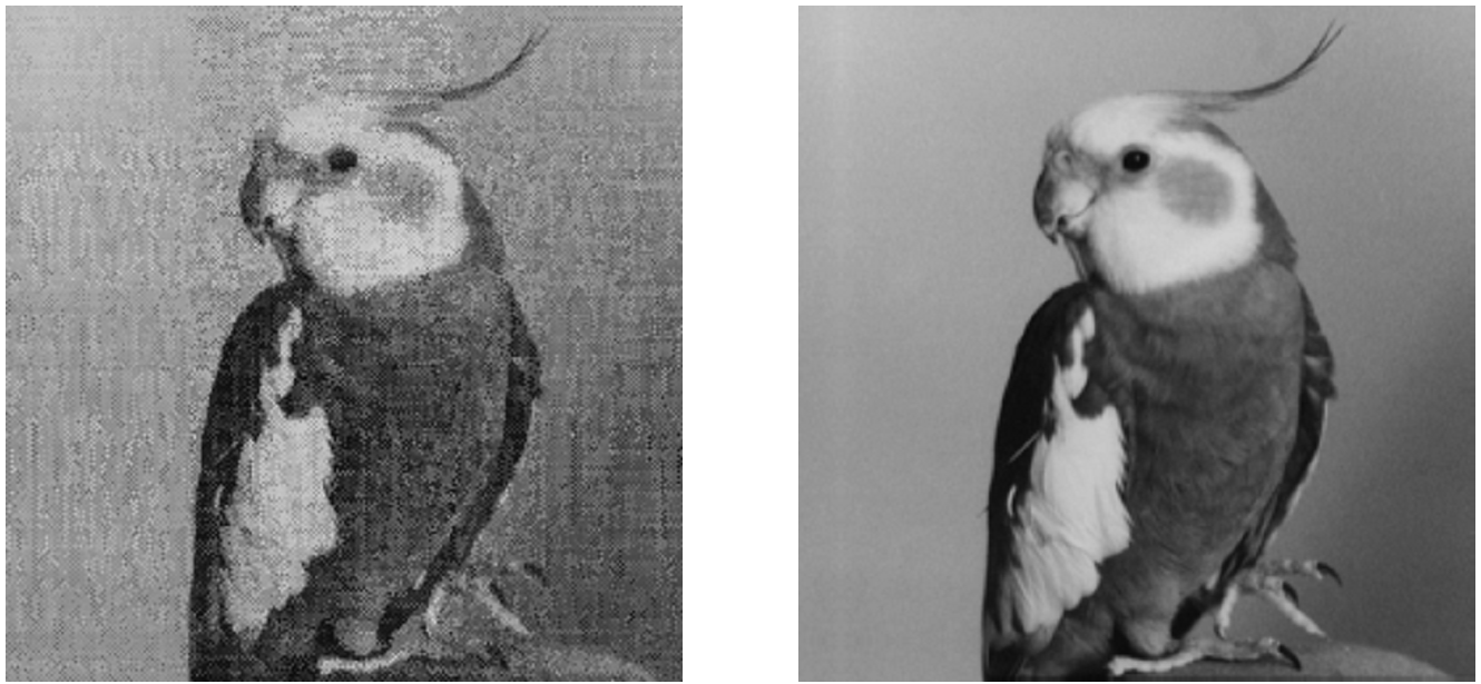
The standard test bird image bird.bmp occupies 66614 bytes. The “compressed” two-dimensional version of the algorithm textual representation of data in the rar archive occupies 10,138 bytes. Quality can be assessed by eye. The point is that I was compressing not a smooth signal, but a photo, which I turned into a “noise”, so that the algorithm could find similar details in it. In reality, if you divide the image into the LF and HF parts, then using conventional smooth algorithms you can compress the LF part and the HF part with the presented algorithm.

I did not refine the idea of ​​software implementation in any language other than the one built into Mathcad, so I used a text format to store data about the compressed image.



Supplement . The reconstructed image of a bird is obtained from a single pseudo-random sequence (PSP). Those. literally all points of the image are derived from the memory bandwidth. The information in this case are the displacements for which you need to take pieces of the "image".

Links

1. Lossy compression algorithm (pdf, many pictures).
2. Archive with documents and calculations (Mathcad).