Welding of optical fibers. Part 4: measurements on optics, removal and analysis of the trace

Two reflectograms of the same path at different wavelengths, opened in the viewer program

Hello! In this, the fourth in a row, article about working with optics, I will talk about how to take a trace reflectogram with an optical reflectometer and how to understand what we see on it. We will also touch on measurement issues with testers, OTDR settings and some others.
The new part did not come out so long, because I wrote a diploma, plus there were questions about the work. But now the diploma is protected, laziness is defeated, and hands have reached to finish the article.

And further. In my personal opinion, this article will seem to the general reader more boring and complex than the previous ones, because it’s one thing to look at fiber welding, and another thing is to dig into some boring graphs. :) But nevertheless, it is necessary to know those who work with optical fiber.
')
Part 1 here
Part 2 here
Part 3 here

Caution: a lot of pictures, traffic!



In the last part, we reviewed the wiring and coupling schemes and the organization of networks, and focused on what kind of reflectometers are, why they are needed, and what they can do. Let's now take a close look at what the measurement result is - the reflectogram , what we can see on it and how to read it.
I'll post images of several typical reflectograms, try to illustrate everything with “live” examples from my practice, but sometimes it may happen that I show something on exemplary imitation schemes drawn in Paint or found on the Internet: just a very long time to collect archives suitable and visual reflectograms for each case.

To work on a computer with reflectograms, I use a program from the manufacturers of reflectometers Yokogawa. She understands the most common format .sor and you can see everything you need in it. I will give a description of its interface and functions at the end of the article. Who wants to try their hand at practice - this is the program . There are several reflectograms in the archive for training. I already gave a link to this archive in the last article.

It must be said that learning to take reflectograms well, analyze them and understand what we see in front of us is more difficult than learning how to solder fibers. There are many nuances. Here you need a lot of practice.
And further. In the last article I gave a link to a large article, which tells everything about reflectometry. Here she is.
Who learns to work with a reflectometer - I advise you not to bypass this material.

To begin with in brief - some important terms.

A trace is a small file of a .sor, .trc format or others, containing a graph - information about the measured track.
Attenuation is a characteristic that indicates how much power (dB or dBm) is lost in a given place (attenuation due to welding, cross) or in this part of the route.
Kilometric attenuation is the attenuation reduced to distance. If we measured and we got the attenuation of the entire line of 0.66 dB and the length of our line is 3 km, then the kilometric will be 0.66 / 3 = 0.22 dB / km.
If any terms in the article are unclear - write in the comments, put it here for clarity. In general, one person can not know everything: clarifications and corrections are welcome.

So, what will we see on the trace when we open it on the instrument or on the computer?
We will see a certain schedule. The abscissa axis shows the distance, the ordinate axis shows the signal power level. In general, the graph is dropping, because everything that is on the optical path causes attenuation to the applied signal: all sorts of connections, defects, and the fiber itself also has a constant attenuation.

A trace is born like this: a reflectometer sends a short pulse of light to a line (its duration is set in the settings), and then it listens to what is reflected back. The fiber itself, due to Rayleigh scattering, slightly reflects back, and, analyzing the power of the back reflection and the time at which this instantaneous power came, the reflectometer puts points on the coordinate plane, connecting them to a graph. If somewhere there is non-reflective heterogeneity (welding, bending), then before it the level of the reflected signal will be higher than after it - a step will appear on the graph. If there is a reflecting heterogeneity (mechanical connection, crack, fiber end), then the reflectometer sees a powerful reflection in this place, much higher than the light coming from Rayleigh scattering - we see a peak on the graph. Since 1 pulse returns very roughly, very noisy, for a high-quality reflectogram many pulses are sent to the line time after time (thousands and tens of thousands), and the resulting trace is their averaging. The more pulses - the more accurate and smoother the trace, but the longer you need to wait for the end of the measurement.

The trace consists of a dead zone at the beginning, a work area and a noise area at the end of the track. Here is the most typical reflectogram in the figure:



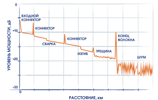
I will refer to this drawing further in the text, so let's designate it as the “main drawing”.

Consider each element on this trace.

At the very beginning there is a peak of the return reflection from the input connector and a loop after it is the so-called dead zone . The length of the track starts from the very beginning of the report scale, that is, the dead zone is already part of the track we are observing. It prevents us from seeing what happens at the very beginning of the route, and this is sad (we cannot directly see if the cross connection is good and whether the pigtail cable is good with the cable). It is impossible to completely get rid of this dead zone, but if you take a series of measures, you can reduce or circumvent it: reduce the pulse duration, use a more sensitive reflectometer, use a compensation coil. And yet we can’t see, say, the welding of the pigtail with the fiber of the cable in the cross, we can say something about it only from indirect data. Indirectly, it is possible to learn about attenuation at the beginning of the route using a compensation coil with fiber (see below).
Much can be said about the state of this dead zone! The cleaner our mechanical connections and the more complete the ends of the patch cords and pigtails, the shorter we set the momentum (see below), the smaller and more accurate this dead zone will be.

If we see that the falling front of the dead zone is in the form of a straight line, and passes into the path at an angle, while the dead zone is neat and narrow (as in the figure above or on the reflectograms from the heading of the article) - everything is set up normally.
If the same, but dead zone is too wide (and other events are wide too), it means that the impulse is too long for this route, the impulse length is too large compared to the length of our section (it’s like trying to loosen the ground in a flower pot with an ordinary shovel) . It is necessary to put a smaller and re-measure the fiber.


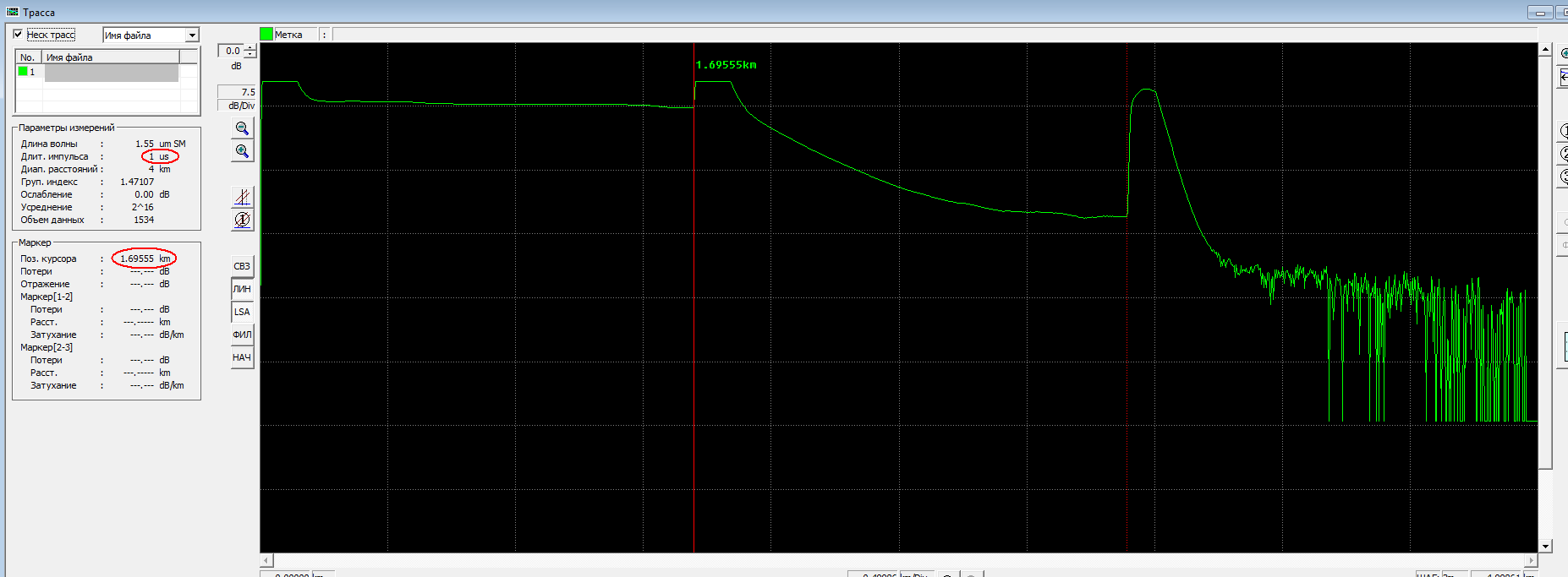
The length of the route is very small (about 1.7 km), and the impulse is too large (1 μs). Therefore, the dead zone and all other events are ugly stretched, "clarity" disappears, small details are lost. For this route you need to set the impulse 100 times shorter. Closer to the right side you can see the phantom peak at twice the distance than the end of the route, see below for details. And another thing: the trace, as you see, is “cut off” in amplitude, the peaks are cut from above. This is already a feature of an inexpensive reflectometer, but this effect usually does not interfere with seeing events on the track.

If the dead zone is not only wide, but goes smoothly into the track (in the form of a hyperbola / parabola), and sometimes even unevenly with noise - this is a sure sign that something is not right at the very beginning of the route: either the ports (on the OTDR or on the cross) are dirty, or the outlet on the cross or on the OTDR itself is broken (in this case, if you disconnect / connect multiple times, the result will vary greatly up to the complete absence of the route), or the patch cord / pigtail is bad, or welding inside the cross is bad. Or, the rarest and most unpleasant option, right near the cross (tens of meters) damage to the cable.
Similar things can be seen in such cases: sometimes when conducting input control of a cable drum (or when it is necessary to measure a line that is not terminated with a cross, there is just a hanging cable end), if there is no device for quick connection (input) of fibers, each fiber has to be welded to the pig- the tail connected to the OTDR, and after taking the measurement, break the welding, weld another fiber, measure again, break, etc. Many solders reasonably save their time and life of the electrodes of the welder, setting the welder so that he curls the fibers, but does not give an arc (Fujikurs allow it, and you can apply a little to the Chinese using the manual mode). At the same time, the OTDR signal goes through a small air gap and, although the route (or the fiber in our cable reel being tested) is clearly visible, the dead zone also often turns out to be not very neat due to the air gap. Although not as terrible as the picture below. In the manual mode, looking at the screen of the welder, it is possible to reduce the fibers very accurately, but still a barely noticeable axial displacement of the fibers already strongly affects the passage of light through the core. Remember that the core of the fiber has a diameter of 9 microns.


See how ugly the beginning of the track? And it happens worse. Most likely, this is a very dirty patch cord on “our” side, but there may be a defect in the optical outlet, cable damage at the cross-country itself, and fiber bending. If this measurement is not from a cross, but by the method described above (when the fibers are reduced to “measure” without welding), maybe the fibers did not come together badly. We turn on the logic: if this is on all the ports of the cross, then our patch cord is bad (or something with a reflectometer socket, or someone cleaned the sockets with something very dirty). If there is 1 fiber and the result is floating from measurement to measurement after reconnection of the patch cord - most likely a defective / broken outlet. If not jumping - maybe bad welding in the cross. If there are several such fibers plus there is no “through fire” at all, it is possible that the cable is damaged near the cross-country or there at the exit from our server / BS. If at 1310 nm is better than at 1550 nm, it is likely that this is a fiber bend in the cross cassette.

At the end of the route, after the final peak, there is an area of ​​noise . This is no longer a track: the track ends with a peak before noises (by the way, if the end of the fiber due to its shape of cleavage or pollution prevents the radiation from reflecting back, the peak at the end of the track may not be or it will be weak, the track will just fall a step into the noise Statistically this happens infrequently, but it happens). The noise area may look different: as a palisade of peaks and dips, or as a flat line along zero, or something in between. I suppose it depends on the processing algorithm and noise drawing by the reflectometer. If the back reflection at the end of the path is strong (the peak is high), then among the noises there can be a phantom peak at a distance twice as large as the length of our path. Its nature is the same as the double reflection of our face from window glass, or the displaced contours of objects on the analog TV screen: electromagnetic radiation flew through the entire fiber and reflected from the end of the track, returned to us (drawing a trace and the main peak), reflected again from our the end of the track, again all the fiber flew away from us, again reflected from the far end, flew to us and only after that got into the OTDR receiver (drawing noises and among the noises a phantom peak). Of course, the losses are great, so this phantom peak, if it makes its way through the noise, it will be much weaker than the peak at the end of the track. And the events of the route itself are not duplicated among the noises never, at least I have not seen this.


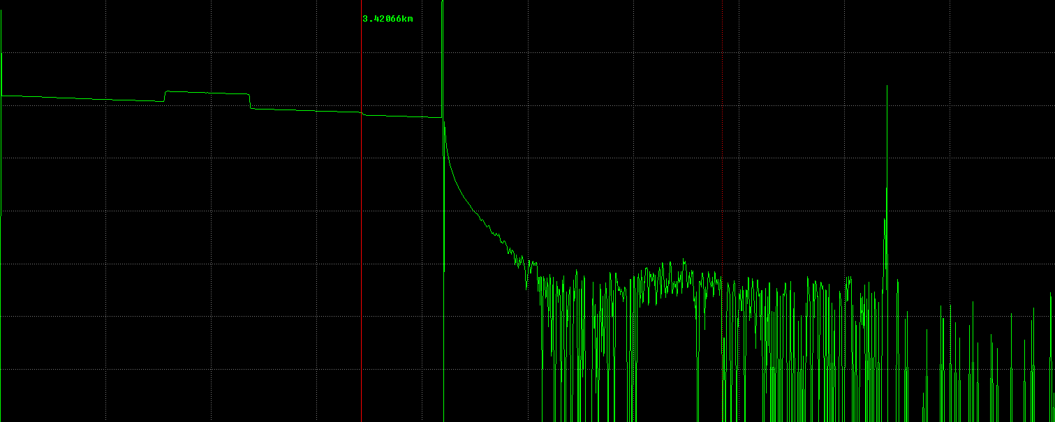
An example of a phantom peak. This route has a length of 6.739 km (I put the red cursor exactly at the end of the route), and at twice the length, among the noises, we see the peak of the reverse reflection. The second pale cursor is an option in the program-viewer of reflectograms just to make sure that this peak is a reflection, and not a real event, programmatically this pale cursor, if the option is on, is always twice as far as the main one. By the way, pay attention to how noise is drawn in this case: a line at zero and small “peaks”.

But between the dead zone and the noise goes the track itself - our working area . In the ideal case (we measure a single piece of cable, without welding and connections), this is a straight line. It has a slope (gradually decreases evenly), since the fiber introduces its own attenuation (in the “transparency windows” of a single-mode fiber, this is not more than 0.22 dB / km (or even less - Wikipedia gives 0.15 dB / km) on the length 1550 nm and not more than 0.36 dB / km at a wavelength of 1310 nm, and usually less, at all other wavelengths, including for visible light, the attenuation is much stronger). This slope is clearly visible in all my pictures with examples of tracks. The shorter the path, the less noticeable the slope (after all, the scale of the long and short trace on the same instrument screen is different), but the slope (with the same scaling by distance) is always about the same and is determined by the attenuation of the fiber.

A small retreat. To whom it is interesting, here is a graph (in two versions), showing the dependence of the attenuation of some optical fiber on the wavelength of the radiation transmitted through it. (Remember that there are a lot of fiber sorts and for each the schedule will be a little different; this is caused by the additives in the glass fiber. I have nothing to tell about these additives, I need a specialist in crystallography and inorganic chemistry). On the graph we see the working areas for our connection - the so-called transparency window ( link to Wikipedia ), where the attenuation is minimal. The first area was used earlier and is now of low relevance (the attenuation is high there), it seems to be used on a multimode. And the second (1310 nm) and third (1550 nm) areas are our workers, therefore, such wavelengths (1310 and 1550 nm) were chosen that the signal could be transmitted farthest to them. For some fibers, there are other areas at a longer wavelength. It is clear that in each transparency window it is possible to organize many separate channels, starting up each at its own wavelength slightly different from the neighboring one: this is how communication systems with wave division (WDM, DWDM) work.





We continue. So, on the ideal route we will see a dead zone, a flat line (the route itself), the end of the route and noises. And what can we see on the working section of the real route, between the dead zone and the end of the route?
a) Welding.
b) Mechanical (cross or fibrlok) connection.
c) Bend the fiber.
d) A crack, not yet turned into a cliff.
d) Open, it is the end of the track.
You can see all these events in the "main figure" above.

On some special expensive reflectometers, we can see something else: for example, a Brillouin reflectometer can show where dangerous mechanical stress is present in the fiber (for example, the sheath and Kevlar cable is ground / burned and it hangs on an honest word and on some fibers, but visually no one has noticed this yet). But we will not touch on these highly specialized and very expensive tools.

Let's start with the difficult.
a) Welding.
How can it look on the trace?
If welding is very good and both welded fibers are the same in properties, it may not be visible at all. With a good welding machine, statistically, there are quite a few such welds, so it happens that in order to find a coupling on the track, you have to look through several reflectograms of different fibers from this line until you get a fiber on which the welding in this coupling is not quite perfect.
In most cases, welding looks like a step down. The larger the step, the greater the damping on it and the worse the welding. You can see the signed weld on the “main figure” above.
How strong is the step acceptable? This is not such a simple question. In general, there are 2 conditions of suitability of the track. The first is that the total attenuation of the path should not exceed the above limits (0.22 dB / km at a wavelength of 1550 nm and 0.36 dB / km at 1310 nm). The second - welding with attenuation of 0.05 dB or less is considered good, if more than 0.05 - apparently, the welding turned out to be defective (there was a bubble, or axial displacement of the fibers in the welder when mixing - see the previous article), and such welding should be digested. (For the method of measuring the attenuation of a signal on irregularities, see below). If after 5 transfusions the attenuation is not better, it is allowed to leave the welding with attenuation no worse than 0.1 dB. So with these two conditions it can be different: for example, we have a difficult route, there are a lot of couplings per unit length (typical for FTTB or for sections where the cable constantly goes from suspension to the ground and back, respectively cable, armor, with Kevlar / cable and on each such transition - a coupling), and in this case, even if we have all welds at 0.05 dB, we can not fit into the standard for kilometric attenuation! This is actually a very unpleasant situation: there are no guilty ones, and there are no bad welds, and the customer may not accept the object, since kilometric attenuation exceeds the norm. It is probably appropriate to ask the designer why he put so many couplings on the line. But he will answer that otherwise the object cannot be built ...
And vice versa: if there are few clutches on a long road (1 clutch per construction length, and the construction length can be 4 and 6 km - depending on how much cable climbs onto the drum), but on one clutch, welding adds> 0.1 dB, in general this fiber can pass the kilometric attenuation rate! But such welding should still be digested.
It is impossible to hammer on bad welds or non-passable fiber! It is better to digest at once than to hope for chance and then go and digest anyway, holding in your hands a list of comments from the customer.

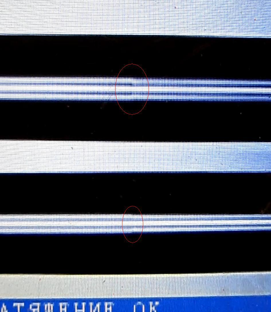
Now more difficult. In some cases, we can see an amazing picture: the step is not down, but up! One might think that in the place of welding the signal is attenuated and amplified. But how is this possible?

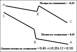
Top left: on the highway, first step up, then step down.

In fact, this gain is imaginary. When measured by testers, only damping will still be there. This situation occurs when two fibers are welded with different refractive indices and different dispersions, usually this is an ordinary SM fiber and some kind of “displaced” (DS or something else). If we measure such welding from both sides of the path, on the one hand there will be a step up, and on the other hand we will see a slightly stronger step down in this place, and the overall average ((A + B) / 2) attenuation will still be positive. By the way, the level of attenuation on the one hand and imaginary amplification on the other can be quite large, up to several decibels (as in the screenshot above), although in fact the attenuation there will be small in both directions. The reason for the imaginary amplification is that the fiber with a displaced dispersion has a slightly different kilometric attenuation, and at the entrance to this section of another fiber, the reflectometer seems to have a gain of some value that is greater than the actual attenuation at that welding, and at the exit of the section it adds the same value to the attenuation in welding, making welding "worse" than it is. The pattern of the appearance of such a step up is approximately visible in this image (different angle of inclination of the straight lines - different kilometric attenuation of glass):



Frankly speaking, I myself do not understand physics and “geometry” with all the depth, why such enormous attenuations and gains can be drawn, even if the insert from the cable with fibers of a different refractive index / dispersion is short. Nevertheless, I come across this quite often, and it is necessary to be able to process such reflectograms with an imaginary gain.
It is clear that in this case it is wrong to judge the quality of welding simply by attenuation (and even more so by reinforcement): if on the one hand imaginary reinforcement is strong, then imaginary attenuation on the other hand will be strong. When there are welding cables with different refractive indices and different dispersions, the attenuation on the welds should be determined only by measuring the path from two sides and calculating the average value. Once again: if cables with different dispersions and generally from different manufacturers are welded, then it is not a fact that bad welding on the trace is really bad! We must look at the other side and take the average value . (The same applies to the definition of kilometric attenuation). Strictly speaking, for conventional welds of the same fibers, this should also be done to increase accuracy, but usually they do not, because accuracy is sufficient in the case of measurement on one side only.
Newcomers sometimes face such a situation: two different cables were welded in the coupling, a trace was taken from one side — and strong attenuation on some fibers. Digested - and the attenuation has not changed. Digested again, and yet, but no use. And if you look at the situation more broadly, in the context of the possibility of imaginary reinforcements and attenuations in welding, and remove reflectograms from the reverse side and calculate the average value for each welding (it is clear that on the reverse reflectogram the sequence of all weldings will be mirrored with respect to the direct reflectogram) , - then everything should be normal. (Although occasionally there are still difficult to explain cases when at least you are bursting, and good welding fails even after 10 digestions by any kind of welder, and on both sides the OTDR draws a significant “step”; I have come across such a couple of times. deviation of geometry / fiber chemistry or something else like that).
Worst of all, some die-hard customers may not know this and insist that it is the hands of the solder and demand to redo the welds, whereas they need to be measured from two sides, calculate the average value and make a start from it. But to hire people for measurements on the one hand, to pay them money is uninteresting, it is much easier to run over connectors and declare them in the curvature of the hands ... :)

Why is it, why do different fibers are boiled at all? Well, for example, by mistake, the suppliers / designers / storekeepers, or because of the lack of an alternative, bought and laid a cable with a part of fibers with a displaced dispersion in the ground, and a regular (or vice versa) cable for suspension, millions of losses and time lost. , , , , , , . , , - «», , ( «» . ). And so on.

, , ( : — , -, -). , , , « » (DWDM, ) , , , - . - , , , .
. , , , . , :



— - , . , , . — , . , Jilong KL-280, - : , ( , , , , ) -, - , , . : , , /..

We continue. ?

) .

, . , « ». , ( — FC/APC, SC/APC, LC/APC, ) . , , ( — 0,1 ; 0,1 — , , , , - -, «» — ). , 1 2 ! -, 2 1 . , .

— , , ( , .. ). ?
, , . - - (FC/APC, SC/APC), , . , . — , , , .
( . ).
, ( , ). , , , (- 0,1 0,02 ).

) .

, , . . 1310 , , 1550 ! , , . , — , - . , , .
— , . - , - , - . , . , : , . , . , - . ? , , «», 4-6 . -, .
, 40 , 60 ( «», ). , , - . — : , , , - . : , , , , , . , . , . ( ), : , , ( , ). !

) . , ( ), ( , - ). , , , . . : , , 1-2 , . , . , - . , . 200-400 , .

) . , — ( — . ). , , . , : . , , .
, , ? : «» . Example. , , , 19,343 , , , 19,107 - , , , , - . :) : , (, ) , , . , , , , , , , . - 2 ( , 2 , , , ).
? 10 , ! : ( ), ( ). , — -4. .

, - ( ) . , : . , . , . — 2 , . () 1310 (, 1310 0,36 /), , — 1550 ( 0,22 /). . .sor- «» , «», «» . , -, — , «» . / («») , . , «» . , , , ( ), , .

APNG- , . (APNG Firefox Presto, , IE ). «» .

( - , APNG , . , , — )

, ! : , - ? .
— 1 .
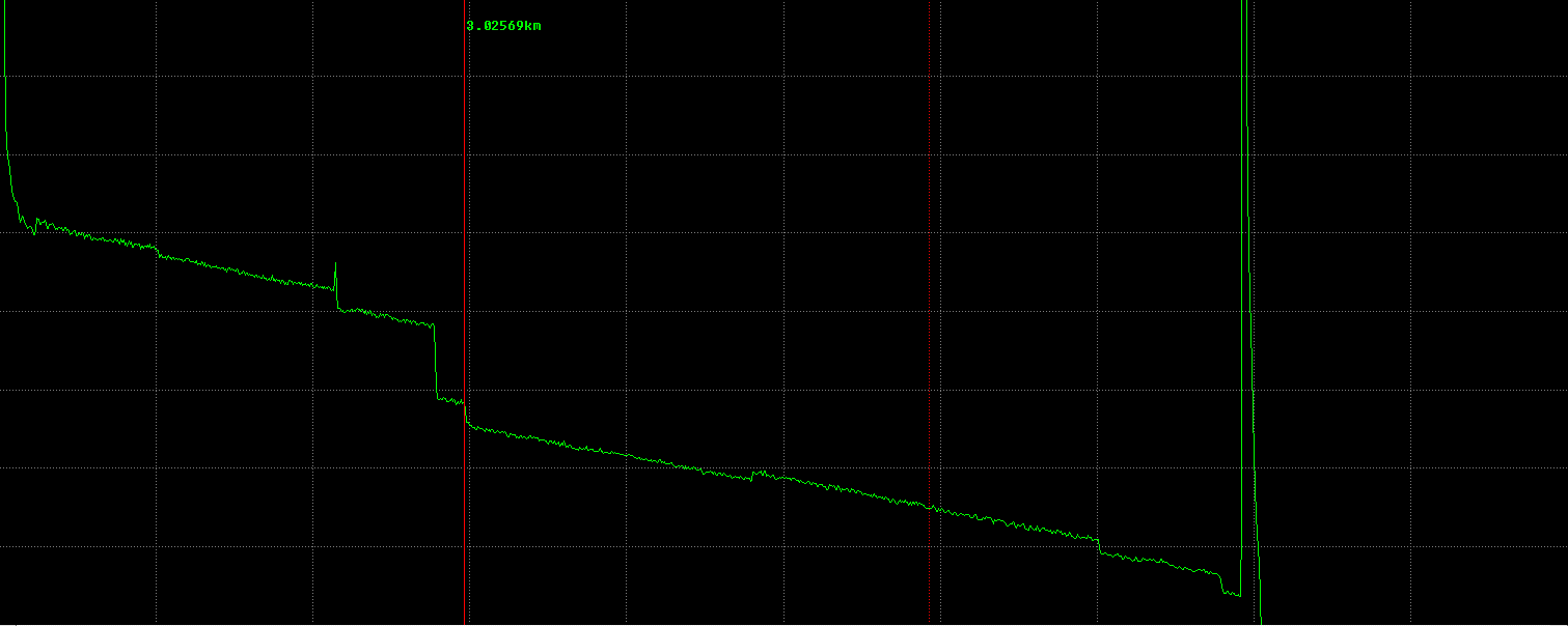
. , 200 , - , , ( - — , , ), . . 2170 ( , , ). — 2,75 — , . 3,025 ( ) . , . , , , , 2 : ( ) 7 — . , «» ( SM, ), ). ( , «» , 3,025 4,8 ). , , . 7,9 , . « », . : , , 1550 , 1310.

, ? .
. , + . , .
«», «». - ( « — - 1 — — - 2 — »).



, . — « », , . , - , - ( — / - !) , — , ( ) . ( ) , - , . — ( /). , . — , . , , , - . , .

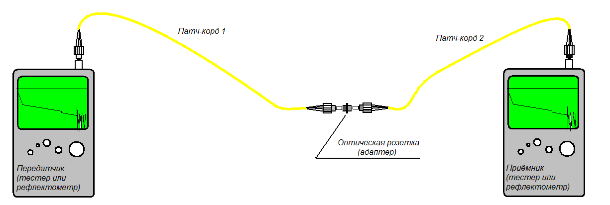
, , , Yokogawa. , , .



.

, , , , , , , -36 /, , , . .

2 . , — () (TPA). () , — . ( , 2 — , , . , — , , ).



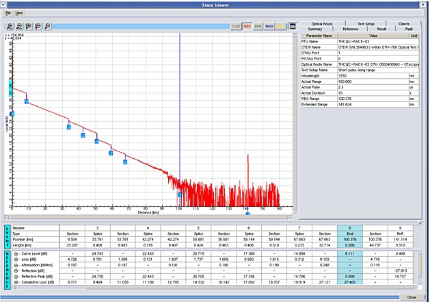
() !The difference of the trace level in these two points is the gross value of the path attenuation in dB; we divide by the optical length between the cursors (markers) - we get the kilometric attenuation (although the instrument or program on the computer can divide and show the result on the fly). Rough - because the reflectogram can be “noisy”, uneven and the height difference of these micro-irregularities can be as high as a few tenths of a decibel and higher. And in the case of a noisy end of a long road at all a catastrophe, this method is not applicable. Here is what a reflectogram looks like at strong zooming (top right - “legend” of a reflectogram, you can see by it which part we zoom in and how):


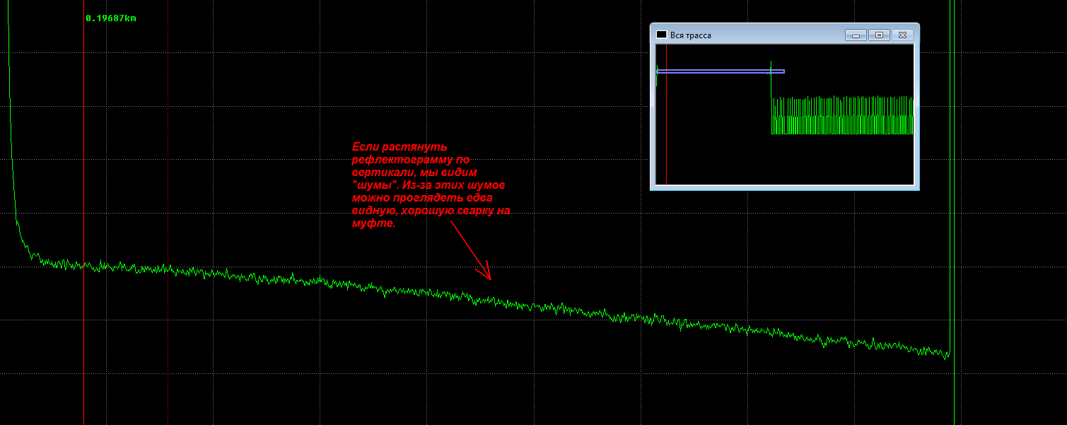
Noise on the trace at high magnification

, , . . , , , . , .

, , .
, — (LSA). , () ( , ), .



, , (). , . , .. - , -, , .
, ! , . How to be? , , , , ( . ), , … , — . : .

. , ( , ), : , , () (, ). , . .

, ( , ).
, : .
(TPA, /) : , — , (, , , SM DS NZ – . ). : , /, , .


1 , 2 — . — . , 0,376 . — . 0,376 — , . , .. .

(LSA, /) , .
. , , -, -, , . : . How to be? . , ( ), , ( — «LSA/TPA» LSA), .


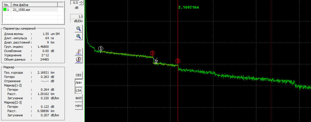
— . , 2 Y2, 0,264 «» — , . , .

, 2 / , ( , , - «Y2») ( «3»)— . , , , ( ), . , : , SM NZ/DS ( ) . . , «» , , , .

, . , .

, . , , . , . - : , . — - , : «», , .

:
1) ( , ),
2) ,
3) / ( ),
4) ,
5) ,
6) .

, , : , , , . , , , - « : /». , , .

, .

1. , , / . , : 300 , 500 , 1 , 2 , 5 , 10 , 25 , 50 , 100 .. , . It's simple. , — , 2 . 2 ? . , : , , , , , , . : , 90% , , - …
: (.. ), (- ): , . ( 50 ), . « — » , .

2. . ( — ), . — . — . — . ? (, , ) , - (). , + , , :


, . - , . , , , .

, , , ( , «» , «» ) Ox. , .



— , .
, : . , 2 . , , - 0,02 , ( 200 ), — , . , , , ! - , , , , . , - . , - . ( , . 200 100 . , .)
? : , , . : , . , .

3. / ( ). , - , . , - , . , - , (, , ). , , , 96 , . .
, , , ( 10000 ) ( 5-10), . 300, - , 1000 ( 10-30 ). , , /. , 1000 , , - , , 5 : 30 ?

, « » . , - ( , , , ) . . . 1 , . ? , «», . , , : ( ) 32 , , , 30 (, , 27 28). , ? : №27 . , , « » . . , , , (, , : , ). , 27 — , ( 30 ). . 28- , , . ( ) , , 5 , , , — .

4. , . ( !). , (, «») . , «» «» . , , . , , 86 325 , . 86 602 ! 300- ( 900-! , !) , . , , .

. — 1,46800, 1,46820.

, , FTTB, , - . - , . , , / . , - . , , 6 , - , , , ( , ), 15 ! , , , , ( ), . , , — - , - .

, . , , , ! — , . , : «4000 , 3999 , 3998 ,… 0 ». — , . , . , . , — , .. , , : , , /, , , . ( ) , . , : , . , , : , - , . , : , , — - . ?..

We continue.
5. Wavelength . Here, too, everything is simple. For single-mode optics, this is 1310 or 1550 nm. For documentation, it is required to take reflectograms at both wavelengths. For myself, in order to better understand that with a line, it’s better at 1550 nm: attenuation is less at this wavelength (we’ll better see the end of the path), and various jambs are seen more clearly, especially such as bends of fibers. By the way! , 1310 , 1550 — , , . 1550 , 1310 — , , . , .

6. . . . , , , , . , , .

( ) — , , . , , . , , .

At last

.

, «» , ? ( OTDR Gamma Lite) . — , , , , - (, ).

, PON, , , ? . :) PON . , , . , PON .

, , - ? : , , ( , ).
, . ( , ), / ( - , ). - , , : , 90- ( , ). , . . , . , :





, .


, 1 , . . ?
, . — -, «» .
, . , , , - , ! Victory? : , , , , — . ? . , . 1 (, 1 — ) , - ( /) ! ! . , . , , , ( , , - , , ). , , - .



, - . - , ( , , , ..). , , .

, . , ( ). , , : , , . - , «». , . : , , (OTDR Gamma Lite), . , , , ? . — , — .

, . , . , , 99,9% , .
, . , , , .

, . , — .
Thank you all for your attention!