Have you ever thought about finding a neat public database, how good would it be to include it in your application in order to optimize any functionality, even if only slightly? Of course! This post will tell you how to use Logstash to turn an external dataset into the desired format, check the result in Kibana and make sure that the data is correctly indexed in Elasticsearch so that it can be used with heavy loads on live servers.

Download data

I will assume that you have already installed the current version of Elasticsearch and Logstash. I will use Elasticsearch 1.1.0 and Logstash 1.4.0 in the following examples.
')
OpenGeoDB is a German website that contains geo-data for Germany in SQL and CSV formats. Since we want to store data in Elasticsearch, then SQL does not suit us, just like CSV. However, despite this, we can use Logstash to convert and index data in Elasticsearch. The file we are going to index contains a list of cities in Germany, including all of their zip codes. This data is available for download from the OpenGeoDB website (download file) under the public domain license.

Data format

After reviewing the data, you can see that they consist of the following columns:

• loc_id: unique identifier (inside the database)
• ags: state administrative code
• ascii: short title in capital letters
• name: entity name
• lat: latitude (coordinates)
• lon: longitude (coordinates)
• amt: not used
• plz: zip code (if more than one, then separated by a comma)
• vorwahl: phone code
• einwohner: population
• flaeche: square
• kz: car license plate series
• typ: type of administrative unit
• level: an integer that determines the location of the area in the hierarchy
• of: terrain identifier of which this locality is
• invalid: column is invalid

We are interested in the name, lat, lon, area, population and license tag fields. We will return to them soon ...

We index entries in Elasticsearch

use csv logstash filter

The next step is to put the data into Elasticsearch. First we set up Logstash. Copy the config below to the opengeodb.conf file. Please note that we use the “csv” filter (comma-separated values), even though the separator is tabulation, not comma.

input { stdin {} } filter { # Step 1, possible dropping if [message] =~ /^#/ { drop {} } # Step 2, splitting csv { # careful... there is a "tab" embedded in the next line: # if you cannot copy paste it, press ctrl+V and then the tab key to create the control sequence # or maybe just tab, depending on your editor separator => ' ' quote_char => '|' # arbitrary, default one is included in the data and does not work columns => [ 'id', 'ags', 'name_uc', 'name', 'lat', 'lon', 'official_description', 'zip', 'phone_area_code', 'population', 'area', 'plate', 'type', 'level', 'of', 'invalid' ] } # Step 3, possible dropping if [level] != '6' { drop {} } # Step 4, zip code splitting if [zip] =~ /,/ { mutate { split => [ "zip", "," ] } } # Step 5, lat/lon love if [lat] and [lon] { # move into own location object for additional geo_point type in ES # copy field, then merge to create array for bettermap mutate { rename => [ "lat", "[location][lat]", "lon", "[location][lon]" ] add_field => { "lonlat" => [ "%{[location][lon]}", "%{[location][lat]}" ] } } } # Step 6, explicit conversion mutate { convert => [ "population", "integer" ] convert => [ "area", "integer" ] convert => [ "[location][lat]", "float" ] convert => [ "[location][lon]", "float" ] convert => [ "[lonlat]", "float" ] } } output { elasticsearch { host => 'localhost' index => 'opengeodb' index_type => "locality" flush_size => 1000 protocol => 'http' } } 

Before continuing, pay attention, this is how we will run Logstash to index the data. Elasticsearch must be running.

 cat DE.tab | logstash-1.4.0/bin/logstash -f opengeodb.conf 

At this stage, quite a lot of things happen (indexing can take a minute or more, it all depends on your equipment). The first thing you can notice is that in the Logstash configuration, input is not used in the “file” instruction. This is because this input method behaves like “tail -f” on UNIX systems, that is, it expects new data to be added to the file. Our file, on the other hand, has a fixed size, so it would be more reasonable to read all its data using the “stdin” input.

The “filter” section consists of six steps. Let's take a closer look at them and explain what each of them does.

step 1 - ignore comments

In the first step, we get rid of comments. They can be identified by the pound symbol at the beginning of a line. This must be done because the first line in our file is just such a comment, which contains the names of the columns. We do not need to index them.

step 2 - disassemble csv

The second step does all the hard work of parsing CSV. You need to override “separator” with “tab” (tab), “quote_char” is one quote by default ”, which is present in the values ​​of our data and therefore must be replaced with another symbol. The“ columns ”property defines the names of the columns that will be used later as field names.

Attention! When copying a file from here, you will need to replace the “separator” character, since instead of a tab, it will be copied as several spaces. If the script does not work as it should, check it first.

step 3 - skip unnecessary records

We need only records that display information about cities (those with a “level” field in the value of 6). We simply ignore the rest of the entries.

step 4 - we process the zip code

The fourth step is needed for proper zip code handling. If a record has more than one zip code (for example, in large cities), they are all contained in one field, but are separated by commas. To save them as an array, rather than one large string, use the “mutate” filter to separate the values ​​of this field. Here, for example, the content of this data in the form of an array of numbers will allow us to use the search for a range of numerical values.

Step 5 - Geo Data Structure

The fifth step will save the geo-data in a more convenient format. When reading from the DE.dat file, separate lat and lon fields are created. However, the meaning of these fields is only when they are stored together. This step writes both fields to two data structures. One looks like the Elasticsearch geo_point type and, as a result, the {"location": {"lat": x, "lon": y}} structure. The other one looks like a simple array and contains longitude (latitude) (in that order!). So we can use the Kibana component bettermap to display the coordinates.

Step 6 - explicit type conversion

The last filter step explicitly assigns data types to some fields. Thus, Elasticsearch will be able to perform numeric operations with them in the future.

The “output” section is only available in Logtash from version 1.4, so make sure you have a version no less. In the previous version you need to explicitly specify the output "elasticsearch_http". Looking ahead, I’ll say that there will be only one “elasticsearch” output and you can specify protocol => http to use HTTP via port 9200 to connect to Elasticsearch.

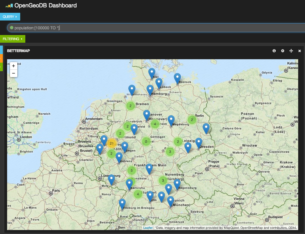
We use Kibana and Elasticsearch for data visualization

When the data is indexed, we can use Kibana for further analysis. Using the bettermap widget and a simple search query like population: [10000 TO *] we can display every big city in Germany.



You can use this, for example, for such purposes:

• Find the cities with the largest population
• Find cities that use a common series of license plates (for example, GT is used in Gütersloh and its surroundings)
• Use the aggregation script to find areas with the most dense or sparse population per square kilometer. You can also pre-calculate these figures in Logstash.

All this is very good, but it does not help us to improve existing applications. We need to go deeper.

Customize autocompletion

Let us digress for a moment and see what useful things you can do with this data. We have cities, postal codes ... and a lot of cases in web applications where you need to enter this particular data.

A good example is the checkout process. Not every store has user data in advance. This may be a store in which orders are often disposable or an order can be made without registration. In this case, it may be appropriate to help the user speed up the checkout process. In this case, the "free" bonus will be to prevent the loss of the order or cancellation due to the complexity of the order.

Elasticsearch has a very fast prefix search functionality called “completion suggester”. But this search has a flaw. You need to slightly supplement your data before indexing, but for this we have Logstash. To better understand this example, you may need to read the introduction to the “completion suggester” (eng).

Tips

Suppose we want to help the user enter the name of the city in which he or she lives. We would also like to provide a list of zip codes to make it easier to find a suitable one for the selected city. You can also do the opposite, first letting the user enter a zip code, and then automatically fill in information about the city.

It's time to make a few changes to the configuration of Logstash to make it work. Let's start with a simple configuration inside the filter. Add this configuration snippet to your opengeodb.conf, immediately after step 5 and before step 6.

  # Step 5 and a half # create a prefix completion field data structure # input can be any of the zips or the name field # weight is the population, so big cities are preferred when the city name is entered mutate { add_field => [ "[suggest][input]", "%{name}" ] add_field => [ "[suggest][output]", "%{name}" ] add_field => [ "[suggest][payload][name]", "%{name}" ] add_field => [ "[suggest][weight]", "%{population}" ] } # add all the zips to the input as well mutate { merge => [ "[suggest][input]", zip ] convert => [ "[suggest][weight]", "integer" ] } # ruby filter to put an array into the event ruby { code => 'event["[suggest][payload][data]"] = event["zip"]' } 

Now Logstash will write the data in a structure that is compatible with the “completion suggester” when it will again index the data. However, you also need to configure the field matching pattern so that the hint function is configured in Elaticsearch. Therefore, you also need to explicitly specify the template in the Logstash settings in the output> elastichsearch section.

 # change the output to this in order to include an index template output { elasticsearch { host => 'localhost' index => 'opengeodb' index_type => "locality" flush_size => 1000 protocol => 'http' template_name => 'opengeodb' template => '/path/to/opengeodb-template.json' } } 

This template is very similar to the default Logstash template, but it includes the suggest and geo_point fields.

 { "template" : "opengeodb", "settings" : { "index.refresh_interval" : "5s" }, "mappings" : { "_default_" : { "_all" : {"enabled" : true}, "dynamic_templates" : [ { "string_fields" : { "match" : "*", "match_mapping_type" : "string", "mapping" : { "type" : "string", "index" : "analyzed", "omit_norms" : true, "fields" : { "raw" : {"type": "string", "index" : "not_analyzed", "ignore_above" : 256} } } } } ], "properties" : { "@version": { "type": "string", "index": "not_analyzed" }, "location" : { "type" : "geo_point" }, "suggest" : { "type": "completion", "payloads" : true, "analyzer" : "whitespace" } } } } } 

Now it's time to delete the old data (including the index) and start re-indexing.

 curl -X DELETE localhost:9200/opengeodb cat DE.tab | logstash-1.4.0/bin/logstash -f opengeodb.conf 

Now you can perform a query to the "sagzhester"

 curl -X GET 'localhost:9200/opengeodb/_suggest?pretty' -d '{ "places" : { "text" : "B", "completion" : { "field" : "suggest" } } }' 

And here is the result:

 { "_shards" : { "total" : 5, "successful" : 5, "failed" : 0 }, "places" : [ { "text" : "B", "offset" : 0, "length" : 1, "options" : [ { "text" : "Berlin", "score" : 3431675.0, "payload" : {"data":["Berlin","10115","10117","10119","10178","10179","10243","10245","10247","10249","10315","10317","10318","10319","10365","10367","10369","10405","10407","10409","10435","10437","10439","10551","10553","10555","10557","10559","10585","10587","10589","10623","10625","10627","10629","10707","10709","10711","10713","10715","10717","10719","10777","10779","10781","10783","10785","10787","10789","10823","10825","10827","10829","10961","10963","10965","10967","10969","10997","10999","12043","12045","12047","12049","12051","12053","12055","12057","12059","12099","12101","12103","12105","12107","12109","12157","12159","12161","12163","12165","12167","12169","12203","12205","12207","12209","12247","12249","12277","12279","12305","12307","12309","12347","12349","12351","12353","12355","12357","12359","12435","12437","12439","12459","12487","12489","12524","12526","12527","12529","12555","12557","12559","12587","12589","12619","12621","12623","12627","12629","12679","12681","12683","12685","12687","12689","13051","13053","13055","13057","13059","13086","13088","13089","13125","13127","13129","13156","13158","13159","13187","13189","13347","13349","13351","13353","13355","13357","13359","13403","13405","13407","13409","13435","13437","13439","13442","13465","13467","13469","13503","13505","13507","13509","13581","13583","13585","13587","13589","13591","13593","13595","13597","13599","13627","13629","14050","14052","14053","14055","14057","14059","14089","14109","14129","14163","14165","14167","14169","14193","14195","14197","14199"]} }, { "text" : "Bremen", "score" : 545932.0, "payload" : {"data":["Bremen","28195","28203","28205","28207","28209","28211","28213","28215","28217","28219","28237","28239","28307","28309","28325","28327","28329","28355","28357","28359","28717","28719","28755","28757","28759","28777","28779","28197","28199","28201","28259","28277","28279"]} }, { "text" : "Bochum", "score" : 388179.0, "payload" : {"data":["Bochum","44787","44789","44791","44793","44795","44797","44799","44801","44803","44805","44807","44809","44866","44867","44869","44879","44892","44894"]} }, { "text" : "Bielefeld", "score" : 328012.0, "payload" : {"data":["Bielefeld","33602","33604","33605","33607","33609","33611","33613","33615","33617","33619","33647","33649","33659","33689","33699","33719","33729","33739"]} }, { "text" : "Bonn", "score" : 311938.0, "payload" : {"data":["Bonn","53111","53113","53115","53117","53119","53121","53123","53125","53127","53129","53173","53175","53177","53179","53225","53227","53229"]} } ] } ] } 

Now, as you may have noticed, it is logical to use the population of the city as its weight. Big cities will be at a higher tip than smaller cities. The returned result contains the name of the city and all its postal codes, which can be used to automatically fill out the form (especially if only one postal code is found).

And that's all for today! However, remember that this is not only suitable for publicly available databases. I am absolutely sure that somewhere, deep inside your company, someone has already collected useful data that are just waiting to be added and used in your applications. Ask your colleagues. You will find such databases in any company.

From translator

This is my first translation. Therefore, thanks in advance to everyone who will help improve it and point out my mistakes.
Thank.