About seals, dogs, machine learning and deep learning
“In 1997, Deep Blue beat Kasparov to chess.
In 2011, Watson furnished the champions Jeopardy.
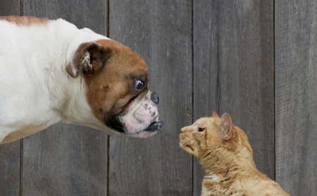
Will your algorithm in 2013 distinguish Bobby from Fluffy? ”
This picture and the preface are from Challenge on Kaggle, which took place last fall. Looking ahead, the last question is quite possible to answer “yes” - a dozen leaders coped with the task by 98.8%, which is surprisingly impressive.
And yet - where does such a question come from? Why were classification problems that a four-year-old child easily solves for a long time (and still remain) too tough for programs? Why is it more difficult to recognize objects of the world than to play chess? What is deep learning and why are seals in the publications about it with frightening consistency? Let's talk about it.
What does it mean to recognize?
Suppose that we have two categories and many, many pictures that need to be decomposed into two groups corresponding to the stack. How are we going to do this? The wonderful answer to this question is that no one knows for sure, but the generally accepted approach is this: we will look for some “interesting” pieces of data in pictures that will be found only in one of the categories. Such pieces of data are called features , and the approach itself is feature detection . There are quite convincing arguments in favor of the fact that the biological brain works somehow - the first thing, of course, is the famous experiment of Hyubel and Wiesel on feline (again) visual cortex cells.
About terms
In the domestic literature about machine learning, instead of feature, they write a “sign”, which, in my opinion, sounds like something vague. Here I will say “feature”, may the Russian language mock me.
')
We never know in advance which parts of our image can be used as good features. In their role can be anything, fragments of the image, shape, size or color. A feature can easily not even be present in the picture itself, but can be expressed in a parameter obtained in some way from the source data - for example, after using the border filter . Ok, let's look at a couple of examples with increasing complexity:
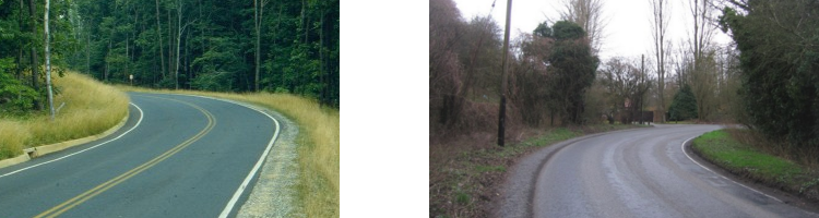
Suppose we want to make a Google car that could distinguish right turns from the left and turn the steering wheel accordingly. The rule for finding a good feature can be thought up almost on the fingers: we cut off the upper half of the picture, select a section of a certain shade (asphalt), apply some logarithmic curve to the left. If all the asphalt fit under the curve - then we have a turn to the right, otherwise - to the left. You can score a few curves in case of turns of different curvature - and, of course, a different set of shades of asphalt, including a dry and wet state. True, on dirt roads, our feature will be useless.
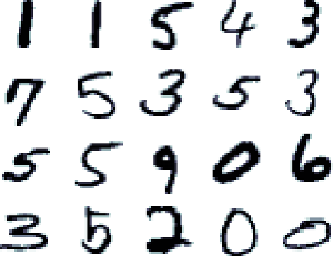
An example from dataset handwritten numbers MNIST - this picture, probably, was seen by anyone who is at least a little familiar with machine learning. Each digit has characteristic geometric elements that define what this digit is - a curl at the bottom of the two, a slash across the entire field of the unit, two docked circles of the figure eight, etc. We can create a set of filters for ourselves that will highlight these essential elements, then apply these filters to our image in turn, and who will show the best result - most likely, this is the correct answer.
These filters will look, for example, like this
Picture from Joffrey Hinton 's course “Neural networks for machine learning”
By the way, pay attention to the numbers 7 and 9 - they have no lower part. The fact is that the sevens and nines are the same, and do not carry any useful information for recognition - so the neural network that developed these features ignored this element. Usually, to obtain such feature filters, we just use ordinary single-layer neural networks or something similar.
Ok, closer to the subject. How about this?
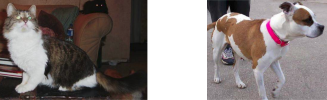
There are a lot of differences between these two pictures - the eyes diverge. The level of brightness, color, or here, for example, a funny coincidence - at the left picture white color prevails in the left part, and at the right one - in the right part. But we need to choose not any, but precisely those that will uniquely identify cats or dogs. That is, for example, the following two pictures should be recognized as belonging to the same category:

If you look at them for a long time and carefully and try to understand what is in common between them, then only the shape of the ears comes to mind - they are more or less the same, just tilted to the right. But this is also a coincidence - you can easily imagine (and find examples from the same data set) a photograph in which the cat looks in the wrong direction, tilts its head, or is generally captured from behind. The rest is all different. The scale, color and length of hair, eyes, posture, background ... Nothing at all in common - and nevertheless, a small device in your head is able to accurately and accurately relate these two pictures to one category, and two ones that are higher - to different . I don’t know how you are, but sometimes I admire that such a powerful device is very close to each of us, only reach out - and yet, we still cannot understand how it works.
Five-minute optimism (and theory)
Okay. But still, if you try to ask a naive question - how do cats visually differ from dogs? We can easily start the list - size, fluffiness, mustache, paw shape, presence of characteristic postures that they can take ... Or, for example, cats have no eyebrows . The problem is that all these distinctive features are not expressed in the language of pixels. We cannot put them into the algorithm until we have previously explained to him what these eyebrows are and where they should be located - or what the legs are and where they grow from. Moreover, we, in general, are doing all these recognition algorithms in order to understand that we have a cat - a creature to which the concepts of "whiskers", "paws" and "tail" are applicable - and before that we don’t even we can say with reasonable confidence where the photo ends in a wallpaper or sofa, and the cat begins. The circle is closed.
But some conclusion from here can still be done. When we formulated features in the previous examples, we proceeded from the possible variability of the object. The turn of the road can only be left or right - there are no other options (except for going straight, of course, but there is nothing to do there), plus the standards of road construction guarantee us that the turn will be quite smooth, and not at a right angle. Therefore, we construct our feature so that it allows different curvature of the turn, a certain set of shades of the road surface, and this is where the possible variability ends. The following example: the number "1" can be written in different handwriting, and all the options will be different from each other - but it must necessarily have a straight vertical (or oblique) bar, otherwise it will cease to be one. When we prepare our feature filter, we leave the classifier room for variability - and if you look at the picture under the spoiler again, you can see that the active part of the filter for the unit is a thick band that allows you to draw a line with a different slope and with a permissible sharp angle at the top.
In the case of cats, the “space for maneuvering” of our objects becomes immeasurably huge. In the picture there can be cats of different breeds, large and small, on any background that one can think of, some object can partially block them, and of course, they can take a hundred thousand different poses - and we have not mentioned the broadcast ( moving the object in the picture to the side), rotation and scaling - the eternal headache of all classifiers. It seems an impossible task to create a flat filter similar to the previous one, which could take into account all these changes - let's try to mentally combine thousands of different forms in one picture, and we will get a shapeless filter spot that will respond positively to everything. Hence, the required features should be some kind of more complex structure. What is not yet clear, but it should be able to take into account all these possible changes in itself.
This “so far incomprehensible” lasted for quite a long time - most of the history of machine learning. But suddenly at some point people understood about the world around them a fascinating idea. It sounds like this:
All things consist of other, smaller and more elementary things.
When I say “all things”, I mean literally anything, anything that we can learn. First of all, since this post about vision is, of course, the objects of the surrounding world depicted in the pictures. Any visible object, we continue the idea, can be represented as a composition of some stable elements, and those in turn consist of geometric shapes, and those are a combination of lines and angles arranged in a specific order. Like this:
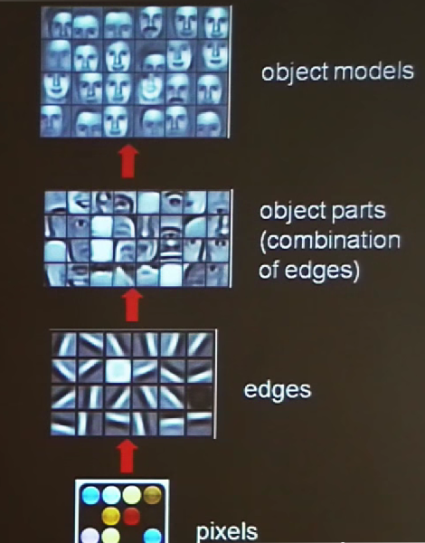
(for some reason I did not find a good informative picture, so this is cut out from the speech of Andrew Un (the founder of Coursera) about deep learning
By the way, within the framework of naive reflections, we can say that our speech and natural language (which have also been considered as questions of artificial intelligence for a long time) is a structural hierarchy, where letters are formed into words, words into phrases, and these, in turn, into sentences and text - and that when we meet with a new word, we don’t have to re-learn all the letters in it, and we don’t perceive unfamiliar texts at all as something that requires special memorization and learning. If you look at the history, you can find many approaches that, to one degree or another (and mostly, much more scientifically based), expressed this idea:
1. Already mentioned, Hubel and Wiesel, in their experiment in 1959, found cells in the visual cortex of the brain that respond to certain characters on the screen — and they also discovered the existence of other cells “higher”, which, in turn, respond to certain stable combinations signals from cells of the first level. Based on this, they assumed the existence of a whole hierarchy of similar detector cells.
a great piece of video from the experiment
... where it is demonstrated how they almost accidentally discovered the necessary feature that made the neuron react — by moving the sample a little further than the usual, so that the edge of the glass fell into the chamber. Sensitive people watch carefully, in the presence of bullying animals.
2. Somewhere in the millennial area among machine-learning specialists, the term deep learning itself appears as applied to neural networks that have more than one layer of neurons, but many - and which, thus, can be trained in several levels of features. Such an architecture has quite strictly justified advantages - the more levels in the network, the more complex functions it can express. Immediately, there is a problem with how to train such networks — the previously used backpropagation algorithm works poorly with a large number of layers. Several different models for this purpose appear - autoencoders, limited Boltzmann machines, etc.
3. Jeff Hawkins, in his book On Intelligence in 2004, writes that a hierarchical approach rules and the future lies with it. He was already a bit late for the beginning of the ball, but I cannot fail to mention him - in the book this idea is derived from completely everyday things and simple language, by a person who was far enough from machine learning and generally said that all these neural networks of yours are bad idea. Read the book, it is very inspiring.
A bit about the codes
So, we have a hypothesis. Instead of stuffing 1024x768 equal pixels into the learning algorithm and watching it slowly suffocating from lack of memory and inability to understand which pixels are important for recognition, we want to extract some hierarchical structure from the picture, which will consist of different levels. At the first level, we expect to see some very basic, structurally simple elements of the picture - its building bricks: borders, strokes, segments. Higher - stable combinations of features of the first level (for example, corners), even higher - features combined from the previous ones (geometric shapes, etc.). Actually, the question is - where to get such a structure for a separate image?
Let’s talk about codes a bit as an abstract question.
When we want to present an object from the real world in a computer, we use some set of rules to translate this object, bit by bit, into a digital form. The letter, for example, is mapped bytes (in ASCII), and the picture is divided into many small pixels, and each of them is expressed by a set of numbers that convey brightness and color information. There are a lot of color representation models, and although, generally speaking, it doesn’t matter what kind of training to use - for simplicity, for now let's imagine a black and white world, where one pixel is represented by a number from 0 to 1, expressing its brightness - from black to white.

What is wrong with this view? Each pixel here is independent, it transmits only a small part of the information about the resulting image. On the one hand, it is pleasant and beneficial when we need to save a picture somewhere or transfer it over the network, because it takes up less space, on the other hand, it is inconvenient for recognition. In our case, we see here an oblique stroke (slightly curved) at the bottom of the image - it is difficult to guess from here, but this is a detail of the outline of the nose from the photo of the face. So, in this case, the pixels that make up this stroke are important to us, the border between black and white is important - and the subtle play of light in shades of light gray at the top of the square is completely unimportant, and you shouldn’t even spend computing resources on it . But in this view we have to deal with all the pixels at once - each of them is no better than the other.
Let's imagine another code now. We decompose this square into a linear sum of other such squares, each of which is multiplied by a coefficient. You can imagine how we take a lot of plates of dark glass with different transparency, and on each plate different strokes are drawn - vertical, horizontal, different. We put these plates stacked on each other, and adjust the transparency so that we get something similar to our drawing - not perfect, but sufficient for recognition purposes.

Our new code consists of functional elements - each of them now says something about the presence of a separate meaningful component in the original square. We see a coefficient of 0.01 for a component with a vertical stroke — and we understand that there is little “verticality” in the sample (but a lot of “oblique stroke” —see the first coefficient). If we independently select the components of this new code, its dictionary, then we can expect that there will be few non-zero coefficients — such a code is called sparse .
The useful properties of this view can be seen in the example of one of the applications called denoising autoencoder . If you take an image, break it up into small squares of size, say, 10x10, and select the appropriate code for each piece - then we can with impressive efficiency then clean this image from random noise and distortion by translating the noisy image into code and restoring it (for example, find, for example, here ). This shows that the code is insensitive to random noise, and retains those parts of the image that we need to perceive the object - so we believe that the noise after the restoration has become “less”.
The downside of this approach is that the new code is heavier - depending on the number of components, the former 10x10 pixel square can weigh in much more. To estimate the scale, there is evidence that the human visual cortex encodes 14x14 pixels (196 dimension) using approximately 100,000 neurons.
And we suddenly got the first level of the hierarchy - it just consists of the dictionary elements of this code, which, as we can now see, are strokes and borders. It remains from somewhere to take this very dictionary.
Five minute practice
We will use the scikit-learn package - a library for machine learning to SciPy (Python). And specifically, the class (surprise) MiniBatchDictionaryLearning. MiniBatch - because the algorithm will not be above the entire dataset at once, but alternately over small, randomly selected data bursts. The process is simple and takes ten lines of code:
from sklearn.decomposition import MiniBatchDictionaryLearning from sklearn.feature_extraction.image import extract_patches_2d from sklearn import preprocessing from scipy.misc import lena lena = lena() / 256.0 # data = extract_patches_2d(lena, (10, 10), max_patches=1000) # 10x10 - data = preprocessing.scale(data.reshape(data.shape[0], -1)) # rescaling - , 1 learning = MiniBatchDictionaryLearning(n_components=49) features = learning.fit(data).components_ If you draw what lies in the features, you get something like the following:
Output via pylab
import pylab as pl for i, feature in enumerate(features): pl.subplot(7, 7, i + 1) pl.imshow(feature.reshape(10, 10), cmap=pl.cm.gray_r, interpolation='nearest') pl.xticks(()) pl.yticks(()) pl.show() 
Here you can briefly stop and remember why we all did it initially. We wanted to get a set of fairly independent from each other "building blocks", from which the imaged object is formed. To achieve this, we cut many, many small square pieces, drove them through an algorithm, and got that all these square pieces can be represented with a sufficient degree of reliability for recognition as a composition of these components. Since at the level of 10x10 pixels (although, of course, it depends on the resolution of the picture), we encounter only edges and borders, we get them as a result, all of them are necessarily different.
We can use this encoded representation as a detector. In order to understand whether a randomly selected piece of a picture is an edge or a border, we take it and ask scikit to find the equivalent code, like this:
patch = lena[0:10, 0:10] code = learning.transform(patch) If any one of the code components has a sufficiently large coefficient compared to the others, then we know that this signals from the presence of a corresponding vertical, horizontal or some other stroke. If all components are about the same, it means that in this place in the picture there is a solid background or noise, which is of no interest to us.
But we want to move on. To do this, you need a few more conversions.
So, any fragment of 10x10 size can now be expressed by a sequence of 49 numbers, each of which will mean the transparency coefficient for the corresponding component in the picture above. And now we take these 49 numbers and write them in the form of a square 7x7 matrix - and draw what we have.
And the following came out (two examples for clarity):
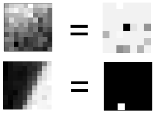
On the left - a fragment of the original image. On the right is its coded representation, where each pixel is the level of the presence of the corresponding component in the code (the lighter, the stronger). It can be noted that the first fragment (upper) does not have a clearly pronounced stroke, and its code looks like a mixture of everything in a weak pale gray intensity, while the second clearly has one component - and the rest are all zero.
Now, to teach the second level of hierarchy, take a larger fragment from the original image (so that several small ones are placed in it - say, 30x30), cut it into small fragments and present each of them in a coded version. Then we dock it back together, and on this data we will train another DictionaryLearning. The logic is simple - if our initial idea is correct, then the adjacent edges and boundaries should also be formed into stable and repetitive combinations.
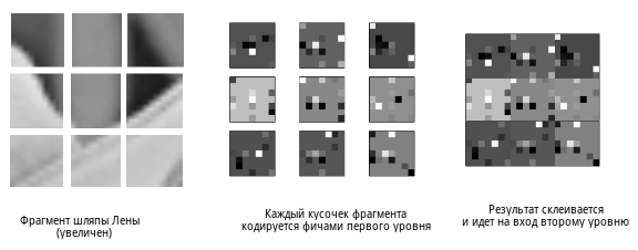
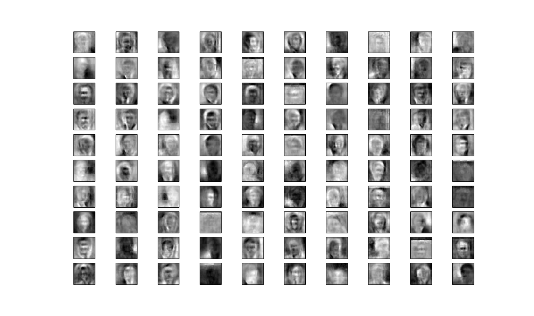
What happened as a result of an example does not seem to be something meaningful at first glance, but this is only by sight. For example, what happens in the second level of the hierarchy that was trained on human faces.
a lot of pictures somehow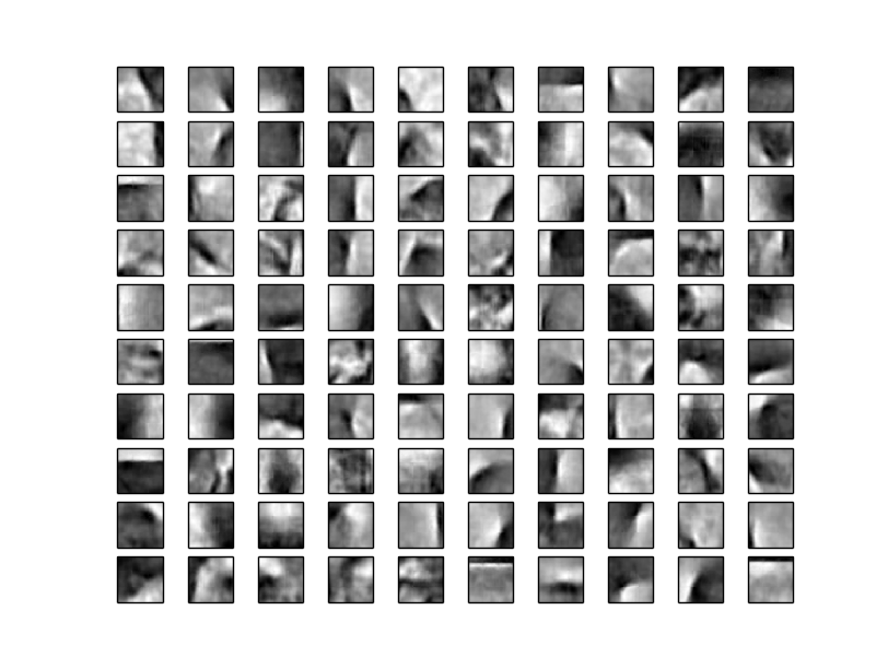
Here, however, the fragment size was chosen more - 25x25 instead of 10x10. One of the unpleasant features of this approach is the need to adjust the size of the “minimum sense unit” yourself.
Here, however, the fragment size was chosen more - 25x25 instead of 10x10. One of the unpleasant features of this approach is the need to adjust the size of the “minimum sense unit” yourself.
Some difficulties arise in order to draw the resulting “dictionary”, because the second level is trained on the code of the first, and its components will look like a motley crochet of dots from the figure above. To do this, we need to take another step down - to break these components into parts again, and “decode” them using the first level, but here we will not consider this process in detail.
And then the levels are increased as long as it is necessary, on exactly the same principle. Here, for example, the third. And here we already see something interesting:
Each face here - feature size 160x160. We have several of the most common locations - front, half a turn to the right and left, plus different skin colors. Moreover, each feature has two more layers below itself, which, firstly, allow you to quickly test test images for validity, and secondly, they give an additional amount of freedom — the outlines and borders can deviate from ideal lines, but as long as they remain within features of their level, they have the opportunity to signal their presence upward.
Not bad.
And what - everything, we won?
Obviously not. In fact, if you run the same script with which I draw all these sets, on the desired dataset about cats and dogs, the picture will be extremely depressing - level by level we will return about the same features, depicting slightly curved borders.
ok that's exactly the last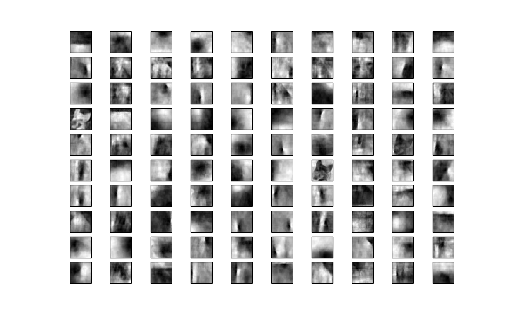
It turned out to catch one dog's face, but this is pure coincidence - because a similar silhouette was encountered in the sample, say, two times. If you run the script again, it may not appear.
It turned out to catch one dog's face, but this is pure coincidence - because a similar silhouette was encountered in the sample, say, two times. If you run the script again, it may not appear.
Our approach suffers because of the same thing that we criticized conventional feed-forward neural networks. In the process of learning, DictionaryLearning tries to search for some common places, structural components of selected fragments of a picture. In the case of faces, everything worked out for us, because they are more or less similar to each other - elongated oval shapes with a certain number of deviations (and several levels of the hierarchy give us more freedom in this regard). In the case of cats, it is no longer possible, because in all the datasets one can hardly find two similar silhouettes. The algorithm does not find anything in common between the pictures in the test sample - excluding the first levels, where we still deal with strokes and borders. Fail Again a dead end.
Ideas for the future
Actually, if you think about it, sampling with a large number of different seals is good in that it covers a variety of breeds, poses, sizes and colors, but it may not be too successful for learning even our intellect. In the end, we learn more by the method of repeated repetitions and observation of an object, rather than by quickly looking through all its possible variations. To learn how to play the piano, we have to constantly play scales - and it would be nice if it would be enough for this to listen to a thousand classic pieces. So, the idea number one is to get away from the diversity in the sample and concentrate on one object in the same scene, but, say, in different positions.
The idea number two comes from the first, and has already been voiced by many, including the one mentioned by Jeff Hawkins, to try to gain from time. In the end, the variety of forms and postures that we see in one object, we see in time - and we can, for a start, group consecutively incoming pictures, assuming that they contain the same cat, just every time several new posture. This means that we, at least, will have to drastically change the training set, and arm ourselves with YouTube videos found at the request of “kitty wakes up”. But about this - in the next series.
Look at the code
... can be on a githaba . Run through python train.py myimage.jpg (you can also specify a folder with pictures), plus additional settings - the number of levels, the size of the fragments, etc. Requires scipy, scikit-learn and matplotlib.
Useful links and what else you can read about intro deep learning
- A Primer on Deep Learning - an informative post with a history of the question, a brief introduction and much more beautiful pictures.
- UFLDL Tutorial - a tutorial from the already mentioned Andrew Ng from Stanford - to get your hands dirty. There is literally everything to get acquainted with how it works - introduction, process math, parallels with feed-forward networks, illustrated examples and exercises in Matlab / Octave.
- The free online book Neural Networks and Deep Learning - unfortunately, is not yet finished. Describes the basics in a fairly popular form, starting with perceptrons, models of neurons, etc.
- Geoffrey Hinton talks about new generations of neural networks
- The last talk with Hawkins , where he briefly expounds about the same as in his book, but more concretely. The fact that an intelligent algorithm should be able to know that the known properties of the human brain tell us about this, what neural networks do not suit us, and what is useful for sparse coding.
Source: https://habr.com/ru/post/226347/
All Articles