Automatic placement of search tags
In this article we will try to talk about the problem of multiple classification on the example of solving the problem of automatic placement of search tags for text documents in our project www.favoraim.com . Readers familiar with the subject will most likely not find anything new for themselves, but in the process of solving this problem we read a lot of different literature where very little was said about the problem of multiple classification, or not at all.
So, let's start with the formulation of the classification problem. Let X be the set of descriptions of objects, Y the set of numbers (or names) of classes. There is an unknown target relationship - mapping whose values are known only on the objects of the final training set
  . Need to build an algorithm
  able to classify an arbitrary object x∈X. However, the most common is the probabilistic formulation of the problem. Let X be the set of descriptions of objects, Y the set of numbers (or names) of classes. On the set of pairs “object, class” X × Y, a probability measure P is defined. There is a finite training set of independent observations obtained according to a probabilistic measure P.
We now turn to the task of automatically placing search tags. We have an object x - a text document and many classes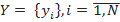 - search tags. Each document must be matched with one or more search tags. For example, we have an event with the title “Concert of the Apocalyptica Group”, this event can be assigned the following search tags: “Apocalyptica”, “concert”, “heavy metal”, “cello”, etc. We also have a training set, i.e. set of documents with already placed search tags. Thus, we have a classification task with overlapping classes, i.e. an object can belong to several classes simultaneously. But instead, we will solve N problems of binary classification, every pair
  we classify into classes {0,1}, i.e. Determine whether you can put a search tag
  x document or not.
To solve this problem, we will present text documents in the form of “bag of words” or a multidimensional vector of words and their weight (frequency) in a document ( http://en.wikipedia.org/wiki/Bag-of-words_model ). In fig. 1 shows a histogram of the words describing business training, in Fig. 2 - a histogram of words describing the master class in photography.
')

As a classification method, you can take any statistical (Bayesian) classification method. The probabilistic model for the classifier is the conditional model p (y│d), y∈Y. Now we need to restore the density p (y│d), y∈Y, i.e. the probability that for our document d you can put the search tag y∈Y. To restore the density, there are many methods, you can start with the naive Bayesian document classification model ( http://ru.wikipedia.org/wiki/Document classification). For this model, a “naive” assumption is made about the independence of the words in the document, and although this is obviously an incorrect assumption, the model works quite well.
Now that we have restored the distribution density and for each tag y∈Y we have found the probability that it can be assigned to our document d, we need to determine which of the tags should be assigned to the document and which should be discarded, i.e. find the minimum cut-off threshold for the probability p (y│d). There will have to use the analysis of the ROC-curve ( http://www.machinelearning.ru/wiki/index.php?title=ROC-curve ).
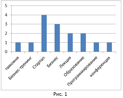
The ROC curve shows the dependence of the number of correctly classified positive examples (true positive rate) on the number of incorrectly classified negative examples (false positive rate). In this case, it is assumed that the classifier has a certain parameter; by varying which, we will receive a particular partition into two classes. This parameter is often called a threshold, or a cut-off point. In our case, the probability p (y│d) will play the role of this parameter. Construct the ROC curve for the control sample, which is usually part of the training sample. In this case, the objects of the control sample can not be used for training the classifier, otherwise we can get an overly optimistic ROC curve due to the phenomenon of retraining. However, if resources allow us, we can use cross-validation. Its essence lies in the fact that the training sample is divided into k parts, k-1 of which are used to train the model, the remaining part is used as a control sample. This procedure is performed k times. In practice, this technique is problematic, because calculations take a lot of time.
The ROC curve has the following main characteristics. Sensitivity (sensitivity) - this is the proportion of truly positive cases. Specificity (specificity) - the proportion of true negative cases that have been correctly identified by the model. Note that fpr = 100-specifity. Area under the ROC curve (AUC). The AUC value is usually used to assess the quality of the classifier. For example, the dependence fpr = tpr corresponds to the worst case (random fortune-telling). In fig. The worst case is indicated by the dotted line. The higher the density, the better the predictions the classifier gives. For an ideal classifier, the ROC curve goes through the top left corner.
Now you need to select the minimum cut-off threshold. There are 3 approaches here.
Thus, we can assign to our document d those search tags for which p (y│d)> c is executed, where c is the value of the cut-off threshold.
And now a little practice. The first thing to do is to convert the text of our document to normal form with the removal of stop words (for example, normalized_string (“example of a string in normal form”) = “example string is a normal form”). For these purposes, postgreSQL FTS dictionaries are quite suitable. Next we need a set of documents with already tagged for training our classifier. As an example, I will cite the pseudo-code for learning the Bayesian naive classifier.
Thus, we assigned to each search tag a histogram of tokens from documents in our training sample. After the classifier is trained, you can proceed to the calculation of the probabilities of the presence of a tag in a new document. In the naive Bayesian model, the probability of the appearance of the tag t for the document d is calculated by the formula , where P (t) is the probability that the tag t occurs,
  - document tokens including repetitions. The probability P (t) can be estimated as
  where
where  Is the number of documents in the training set with the t tag, and N is the number of all documents in the training set. Estimation of probabilities P (l│t) with the help of the training set is as follows
  where
where  - the number of occurrences of the lexeme l in all documents with the tag t, and
  - the number of all tokens in all documents with a tag t. To avoid overflow in the formula for calculating probabilities due to the large number of factors, in practice, instead of the product, the sum of logarithms is usually used. Logarithm does not affect the finding of the maximum, since the logarithm is a monotonically increasing function.
It remains to construct the ROC curve. As a pseudocode, I, perhaps, will insert copy-paste.
To search for the cut-off threshold by default, it is proposed to choose method 2: the requirement of the maximum total sensitivity and specificity of the model, I think it will not be difficult to find it. That's probably all, if you have questions or suggestions, write, I will be happy to answer them.
So, let's start with the formulation of the classification problem. Let X be the set of descriptions of objects, Y the set of numbers (or names) of classes. There is an unknown target relationship - mapping
whose values are known only on the objects of the final training set . Need to build an algorithm able to classify an arbitrary object x∈X. However, the most common is the probabilistic formulation of the problem. Let X be the set of descriptions of objects, Y the set of numbers (or names) of classes. On the set of pairs “object, class” X × Y, a probability measure P is defined. There is a finite training set of independent observations obtained according to a probabilistic measure P.We now turn to the task of automatically placing search tags. We have an object x - a text document and many classes
- search tags. Each document must be matched with one or more search tags. For example, we have an event with the title “Concert of the Apocalyptica Group”, this event can be assigned the following search tags: “Apocalyptica”, “concert”, “heavy metal”, “cello”, etc. We also have a training set, i.e. set of documents with already placed search tags. Thus, we have a classification task with overlapping classes, i.e. an object can belong to several classes simultaneously. But instead, we will solve N problems of binary classification, every pair we classify into classes {0,1}, i.e. Determine whether you can put a search tag x document or not.To solve this problem, we will present text documents in the form of “bag of words” or a multidimensional vector of words and their weight (frequency) in a document ( http://en.wikipedia.org/wiki/Bag-of-words_model ). In fig. 1 shows a histogram of the words describing business training, in Fig. 2 - a histogram of words describing the master class in photography.
')
As a classification method, you can take any statistical (Bayesian) classification method. The probabilistic model for the classifier is the conditional model p (y│d), y∈Y. Now we need to restore the density p (y│d), y∈Y, i.e. the probability that for our document d you can put the search tag y∈Y. To restore the density, there are many methods, you can start with the naive Bayesian document classification model ( http://ru.wikipedia.org/wiki/Document classification). For this model, a “naive” assumption is made about the independence of the words in the document, and although this is obviously an incorrect assumption, the model works quite well.
Now that we have restored the distribution density and for each tag y∈Y we have found the probability that it can be assigned to our document d, we need to determine which of the tags should be assigned to the document and which should be discarded, i.e. find the minimum cut-off threshold for the probability p (y│d). There will have to use the analysis of the ROC-curve ( http://www.machinelearning.ru/wiki/index.php?title=ROC-curve ).
The ROC curve shows the dependence of the number of correctly classified positive examples (true positive rate) on the number of incorrectly classified negative examples (false positive rate). In this case, it is assumed that the classifier has a certain parameter; by varying which, we will receive a particular partition into two classes. This parameter is often called a threshold, or a cut-off point. In our case, the probability p (y│d) will play the role of this parameter. Construct the ROC curve for the control sample, which is usually part of the training sample. In this case, the objects of the control sample can not be used for training the classifier, otherwise we can get an overly optimistic ROC curve due to the phenomenon of retraining. However, if resources allow us, we can use cross-validation. Its essence lies in the fact that the training sample is divided into k parts, k-1 of which are used to train the model, the remaining part is used as a control sample. This procedure is performed k times. In practice, this technique is problematic, because calculations take a lot of time.
The ROC curve has the following main characteristics. Sensitivity (sensitivity) - this is the proportion of truly positive cases. Specificity (specificity) - the proportion of true negative cases that have been correctly identified by the model. Note that fpr = 100-specifity. Area under the ROC curve (AUC). The AUC value is usually used to assess the quality of the classifier. For example, the dependence fpr = tpr corresponds to the worst case (random fortune-telling). In fig. The worst case is indicated by the dotted line. The higher the density, the better the predictions the classifier gives. For an ideal classifier, the ROC curve goes through the top left corner.
Now you need to select the minimum cut-off threshold. There are 3 approaches here.
- The requirement of the minimum value of the sensitivity (specificity) of the model. Those. one of the values is set constant and, based on this, the value of the cut-off threshold is selected.
- The requirement of the maximum total sensitivity and specificity of the model.
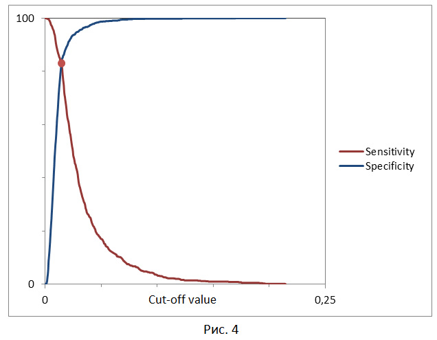
- The requirement of a balance between sensitivity and specificity, i.e. when specificity≈sensivity. Here the threshold is the intersection point of the two curves, when the cut-off threshold is plotted along the x axis, and the sensitivity and specificity of the model along the y axis (Fig. 4).
Thus, we can assign to our document d those search tags for which p (y│d)> c is executed, where c is the value of the cut-off threshold.
And now a little practice. The first thing to do is to convert the text of our document to normal form with the removal of stop words (for example, normalized_string (“example of a string in normal form”) = “example string is a normal form”). For these purposes, postgreSQL FTS dictionaries are quite suitable. Next we need a set of documents with already tagged for training our classifier. As an example, I will cite the pseudo-code for learning the Bayesian naive classifier.
Map<String, Map<String, Integer>> naiveBayes; for (Entry<String, String[]> entry: docSet) { for (String lexem: get_normalized_string(entry.key).split(MY_DELIMS)) { for (String tag: entry.value) { naiveBayes[tag][lexem]++; } } } Thus, we assigned to each search tag a histogram of tokens from documents in our training sample. After the classifier is trained, you can proceed to the calculation of the probabilities of the presence of a tag in a new document. In the naive Bayesian model, the probability of the appearance of the tag t for the document d is calculated by the formula
, where P (t) is the probability that the tag t occurs, - document tokens including repetitions. The probability P (t) can be estimated as where Is the number of documents in the training set with the t tag, and N is the number of all documents in the training set. Estimation of probabilities P (l│t) with the help of the training set is as follows where - the number of occurrences of the lexeme l in all documents with the tag t, and - the number of all tokens in all documents with a tag t. To avoid overflow in the formula for calculating probabilities due to the large number of factors, in practice, instead of the product, the sum of logarithms is usually used. Logarithm does not affect the finding of the maximum, since the logarithm is a monotonically increasing function. Map<String, Double> probs; for (String tag: naiveBayes.keySet()) { probs[tag] = log(P(t)); for (String lexem: get_normalized_string(document).split(MY_DELIMS)) { probs[tag] += log(naiveBayes[tag][lexem]/sum(naiveBayes[tag])); } } It remains to construct the ROC curve. As a pseudocode, I, perhaps, will insert copy-paste.
Canonical ROC curve construction algorithm
Inputs: L - many examples; f [i] is the rating obtained by the model, or the probability that the i-th example has a positive outcome; min and max are the minimum and maximum values returned by f; dx - step; P and N are the number of positive and negative examples, respectively.t=min FP=TP=0 i L { f[i] >= t // i { TP=TP+1 } // { FP=FP+1 } } Se=TP/P*100 100_m_Sp=FP/N // (100 Sp) (100_m_Sp, Se) ROC t=t+dx (t>max)
To search for the cut-off threshold by default, it is proposed to choose method 2: the requirement of the maximum total sensitivity and specificity of the model, I think it will not be difficult to find it. That's probably all, if you have questions or suggestions, write, I will be happy to answer them.
Source: https://habr.com/ru/post/222731/
All Articles