Inverse kinematics: simple and fast algorithm

What is Inverse Kinematics?

The task of inverse kinematics is the search for such a set of articulation configurations that would ensure the most gentle, fast and accurate movement to the specified points. However, many methods currently existing suffer from such disadvantages as high computational complexity and unnaturalness of the resulting postures. This article describes a new ( probably, at the time of writing the article - 2010 ) heuristic method called Forward and Backward Reverse Method ( Forward and Backward Reaching Inverse Kinematics , hereinafter simply FABRIK),
FABRIK avoids the use of rotations and matrices in favor of directly obtaining a point on a straight line. Due to this, the matter costs only a few iterations, has a low computation cost and a visually natural posture as a result. FABRIK also cope with the imposition of restrictions as well as the use of multiple chains and / or end points. It is about this method of this post.


I ask you to treat this squeeze with understanding, because the original is quite large, has a lot of water, relevant and inappropriate repetitions and separations from the topic, as well as comparisons with other algorithms. I decided to nevertheless neglect this, therefore, here there is only a small part of the text, which, however, reflects the essence - approx. trans.
')

1. Artificial body model

A system of many solids consists of a set of solids, called nodes, connected together by edges. All edges are components associated with motion: they restrict movement within a certain angle relative to adjacent edges. Virtual body modeling is important for calculating a person’s posture. A model with properly placed restrictions will allow you to get a set of correct poses, which will give you the opportunity to get a more realistic movement. Most models imply the hardness of body parts, although this is just an approximate approximation to reality.
The skeleton is usually modeled as a hierarchy of solid segments connected by edges, each of which is given by such properties as length, shape, volume and mass. The manipulator, in the manner of a robo-arm or an animated character, is modeled as a chain, assembled from solid knots, conjugated with each other by edges. Each movement and / or rotation of the bone with the index i affects all subsequent elements of the chain. A chain can be formalized as follows: every node without children should be the end point; for each end point, the chain can be formed backward in the skeleton, from parent to parent, until the root node of the chain (the beginning of the chain) is encountered. By definition, the IK problem assumes that the root node is static. However, methods usually cope with the movement of the root.

2.FABRIK - a new heuristic solution of the IK problem

This section provides the essence of the FABRIK method. It uses positions already calculated in forward and reverse modes. FABRIK minimizes the error by adjusting the angle of each node once. Those. the whole chain is traversed, starting from the last node, with adjustment of the angle of each bypass node, after which the chain is already traversed in the opposite direction. This method, in contrast to the transformation of rotations, turns the problem of finding the position of a node into the problem of finding a point on a line; therefore, you can save time and reduce the number of calculations. Suppose that the set p [1], ..., p [n] is the set of positions of the nodes of the manipulator. Also, suppose that p [1] is a root node and p [n] is an end node, so for simplicity, leave one end node. The target is represented by the position t and the initial base position b . The FABRIK method is shown in the listing above and in the graphical interpretation of the complete cycle in the figure to the left, with one target point and four nodes in the circuit. Consider the full cycle of the algorithm in the figure:

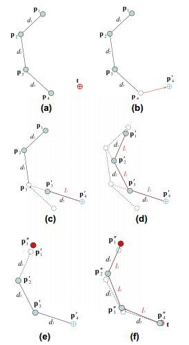
• a - The initial positions of the manipulator and the target.
  
• b - Move end node p [4] to the target.
  
• c - We find the position of p '[3] , lying on the line between the positions of p' [4] and p [3] , at a distance d [3] from point p '[4] .
  
• d - Repeat for all nodes.
  
• e - The second stage of the algorithm: move the root element from the position p '[1] to its initial position.
  
• f - Repeat for all nodes, but this time we start from the base and move to the end node. The algorithm is repeated until the position of the final element is close to the target for a sufficient distance.
  

In details:
First, the positions between the nodes are considered (array d ), after which it is checked whether the target point is reachable; the distance between the root node and the target ( dist ) is considered, and if this distance is less than the total sum of the distances between the nodes, then the goal is achievable, otherwise there is no. If the goal is attainable, the full cycle is limited to two stages. At the first stage, the algorithm estimates the initial position of each node, starting from the final element p [n] moving to the base of the manipulator p [1] . Thus, let the target position be the position of the end node, p '[n] = t . We obtain the line l [n-1] lying on the points p [n-1] and p '[n] . The new position of the node with the index n-1 , p '[n-1] , lies on this line at a distance d [n-1] from p' [n] . Similarly, the new position of the node with the index n-2 , p '[n-2] , can be calculated using the straight line l [n-2] lying on the points p [n-2] and p' [n-1] at a distance d [n-2] from p '[n-1] . The algorithm is repeated until all new positions are calculated for all nodes, including the final one. In cases where the root element moves to the desired position, FABRIK operates as described, with the only difference that the new position p '' [1] of the root node will be the desired position, not the initial one.
After one complete iteration, in almost all cases (as observed), the end node will approach the target. The procedure will be repeated as many times as necessary, until the end node lies on the target position or approaches it at the allowable distance. Implementation of the FABRIK method without introducing limiters will converge at any target point / chain if the goal is attainable. However, if the target is further than the reach to which the chain can stretch, an interrupting condition is needed that compares the past and current position of the end node, and which terminates the algorithm if the end node offset is less than a certain value (epsilon). Also, in special cases, the algorithm is interrupted after a certain number of iterations (however, such a situation has not yet been encountered).
For faster results and solutions in several iterations, optimization with the use of Conformal Geometric Algebra (hereinafter CGA) is possible; CGA has an advantage on basic shapes, such as spheres, straight lines, planes and circles, which are fairly simply displayed by algebraic objects. Therefore, the search for the position of a node located between two known nodes can be expressed by the intersection of two spheres with the centers at the corresponding positions of these nodes, and a radius equal to the distance between the positions of the desired node and the existing ones; The new position of the node will lie on the nearest point of the circle formed by the intersection of the two spheres. Another simple optimization is the direct construction of a straight line in the direction of the goal, when the latter is not available.

3. Model with multiple end nodes

As in the case of a single end node, the algorithm is divided into two stages:

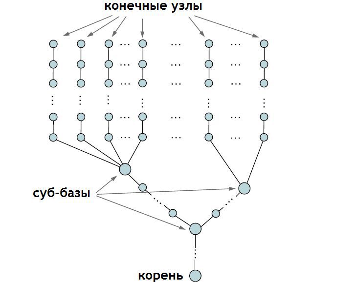
• The first stage is exactly the same, only this time it starts from each end node with movement inwards along the chain from this node, up to the sub-base (probably the sub-base is a node with several adjacent edges - approx. Transl.) . Thus, we will get as many different positions for a subbase as we have end nodes connected to it. The total position can be taken as a centroid (tobish, just the arithmetic mean - approx. Transl.) From these positions. After that, the execution of the algorithm continues in the normal mode, moving from the sub-base to the root. If sub-bases have their own sub-bases, then similar actions are performed on them - a list of possible positions is also compiled, after which this sub-base is set to a centroid from the entire list of positions.
  
• At the second stage, the usual algorithm is applied to each node, moving further away from the root node. At the same time, each chain must be processed separately up to the end node: the more sub-bases, the more repetitions for each of them. The process is repeated until the end nodes reach their goal or until the interrupt condition is triggered.
  

4. Limiters

And finally, the most tasty part of this article is calculations using limiters. They are needed, as it was worth guessing, for greater similarity with real organisms. The node itself is usually characterized by three degrees of freedom. Rotation of a node can be characterized as “simple rotation” (2 degrees of freedom), which reflects its final position, and rotation around its own axis (1 degree of freedom). Thus, by dividing the movement of a node into two such phases, and applying constraints to them, you can control the position of the node. The restrictions themselves can be imposed in a similar way: the algorithm is iterative, it is possible to apply rotation restrictions at each iteration of the algorithm. Limiters, however, will not affect the convergence of the algorithm. The main idea of ​​using limiters is to reposition and reorient nodes within limits.

• a - Initial manipulator and target configurations.
  
• b - Move the end node p [4] to the target and orient it to it.
  
• c - We find the position of p '[3] , lying on the line between the positions of p' [4] and p [3] , at a distance d [3] from point p '[4] .
  
• d - Reorient the node at position p '[3] so that it looks along the edge connecting p' [3] and p '[4] .
  
• e - Calculate bounding ellipse: the allowed positions are in the shaded area. None of the vertices at this stage moves anywhere.
  
• f - The node p [2] moves to the position p ^ [2] , which is the closest position on the shaded ellipse, thus making sure that the new position p ^ [2] will lie within acceptable limits.
  
• g - Move the node p ^ [2] to the point p '[2] in order to maintain the length of the edge.
  
• h - Reorient p '[2] to satisfy constraint orientation.
  

This procedure is repeated for all nodes, in the direct and reverse order, in the same way as in the unrestricted version of the movement. At the same time, the “ellipse” constraint is probably a characteristic of an edge, not a node, that is, in the second phase, the p [3] node should move into an ellipse - approx. trans.