The task of changing the voice. Part 3. Applied speech signal models: LPC

We continue the cycle of articles devoted to the task of changing the human voice, on the solution of which we work in the company i-Free . In the previous article I tried to briefly describe the mathematical apparatus used to describe complex physical processes occurring in a person’s vocal tract when pronouncing sounds. Issues related to the modeling of the acoustics of the vocal tract were raised. Admissible simplifications and approximations were described. The result of the article was the reduction of the physical model of sound propagation in the speech path to a simple discrete filter.

In this article, on the one hand, it would be desirable to continue the previous undertakings, and on the other, to move away a bit from the fundamental theory and talk about more practical (more “engineering”) things. One of the applied models that is often used when working with a speech signal will be briefly considered. The mathematical basis of this approach, as is often the case, was originally laid as part of a completely different research. Nevertheless, the physical features of the speech signal made it possible to apply these ideas precisely for its effective analysis and modification.
')
The previous article, due to the specifics of the issue under consideration, was oversaturated with scientific terms and formulas. In this one, we will try, instead of a detailed description of mathematical constructions, to focus on the ideological concept and the qualitative characteristics of the model being described.

The theory of the LPC (Linear Prediction Coding) model will be discussed in more detail - a remarkable slender approach to describing the speech signal, which in the past determined the direction of speech technology development for several decades and is still often used as one of the basic tools for analyzing and describing the speech signal .

Simplified discrete speech model

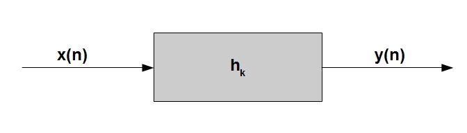
In this section , we will make the transition from the discrete model of the vocal tract from the previous article (that model described only the propagation of sound in pipes with a constant cross-sectional area), to a more complete model describing the entire articulation process. The basic idea of ​​the model is formulated quite simply - let us imagine that the discrete signal y (n) * analyzed by us is the output of a linear digital filter a ** h, through which a certain “exciting” signal x (n) passes:
_____________________________
* - hereinafter we will talk only about discrete signals and the time variable t will be replaced with a discrete reference index n
** - we immediately apologize for some references to English-language sources, but often they contain the required question more fully and in one place, we hope the language barrier will not be a big obstacle.



It is logical to assume that by changing the filter coefficients h_k, and, perhaps, in some cases, the “exciting” signal itself, you can achieve a different sound of the output sound *. In words, everything is quite simple, but now we will try to figure out what relation this completely abstract generalized idea may have to a speech signal.
_____________________________
* - as in the previous article, the symbol "_" we will denote the indexing operation, and the symbol "^" - the operation of raising to a power.

We briefly recall, but at the same time we summarize a little of what was told in the very first article . The formation of speech sounds can, with some reservations, be described as follows:

1) the glottis in the larynx is a “basic” sound source (here, with the participation of the vocal cords, the same vocalized or unvoiced excitation signal from Section 1 is generated)

2) the organs of the vocal tract above the larynx are one complex acoustic filter that strengthens one and weakens other frequencies

3) “the final touch” to the final sound adds the process of emission of sound waves by mouth or nose

The last point can be neglected to some extent, since This transformation above the signal can be approximated by differentiation and, accordingly, it is relatively easy to reverse its effect on the signal. With the first two the story is somewhat more complicated. Both process data are not stationary in time. When generating a voiced excitation signal, the period of closure and the degree of closure of the folds of the glottis in the larynx continuously change, which causes a change in the duration and in the form of "guttural" air pulses: as a result, the intonation and sound intensity, emotional color of speech changes. The speech path above the larynx is one large moving acoustic filter; its chambers and connections, changing their geometry, change the position of the resonant (formant) and antiresonant frequencies — the type of pronounced vocalized sound changes in terms of phonetics. When pronouncing unvoiced sound, vocal folds do not work, and the larynx is the source of the noise signal. The work of the rest of the vocal tract does not fundamentally change and, as a result, the spectrum of noisy speech sounds also has a formant structure, albeit somewhat less “noticeable.” The above can be illustrated by the following simplified scheme:



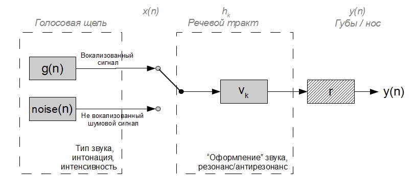
Corresponding elements from the 1st figure are indicated in gray font at the top.

In real life, there are a lot of nuances and mechanisms of the mutual influence of the vocal tract on the larynx and vice versa, as well as the breathing apparatus on the entire acoustics of the vocal tract at the moment when the speech gap is open. However, considering several “idealized” processes, we can say that this picture adapts the previous abstract idea “excitation signal - filter - sound” to the articulation of speech sounds and at the same time takes into account the basic properties of a real speech signal quite well.

The advantages of this look at the process of sound formation:

- the ability to consider the signal of excitation of the vocal tract and its further distribution along the vocal tract independently of each other (in fact, they are nevertheless interconnected, however, this interrelation is not always clearly expressed and in some cases it can be neglected)

- the ability to analyze the vocal tract as a linear stationary (at short time intervals) system

- the ability to well approximate most of the sounds in the speech signal

Of course, as is always the case in real life, this simplified approach is not so simple for practical use. Many uncertainties arise even at the stage of splitting the analyzed signal into voiced / unvoiced segments. Only for this task, in general, is it necessary to carry out a complex signal processing involving a serious mate. apparatus. The next difficult point is the nonstationarity of the processes under consideration, and in this case x (n) changes much more rapidly than h (n). To obtain reliable estimates of the parameters of this model, the most optimal is signal processing on time segments, the duration of which is a multiple of the pitch period, which is not easy, given that this period is constantly changing. It is also worth mentioning the limited applicability of this model for describing some consonant sounds, in particular fricative and “explosive” ones. When pronouncing a ringing fricative sound, the voiced excitation signal passes through a significant contraction in one or another part of the vocal tract, which leads to the formation of strong turbulent noise. A deaf fricative is pronounced similarly, with the difference that the exciting signal is initially noisy. Thus, the noise component of fricative sounds is largely formed already in the vocal tract, and not only in the larynx, which is not taken into account by this model. “Explosive” sounds are a special case, the consideration of which we have so far omitted.

We now turn from a generalized discrete model to concrete applied models, which allow one to estimate certain parameters of a speech signal.

Linear Prediction Coefficients (Linear Prediction Coding Coefficients or simply LPC)

The LPC method is a simple approach to the generalized discrete model of a speech signal described above. Namely, the LPC coefficients directly describe the V speech path (see the previous figure). This description is of course not exhaustive and is a kind of approximation of a real speaker system. However, as claimed by the theory, and as many times proved by practice (take at least the CELP algorithms used in modern cellular networks), this approximation is quite sufficient for many, many cases. The white spot in the LPC model is the signal of the excitation of the vocal tract, which in practice either does not change significantly, or, for example, is replaced with some previously calculated one, as in CELP.

We describe in more formal terms exactly what place the LPC coefficients occupy in the system under consideration. The signal at the input of the vocal tract (at the exit of the glottis) will be referred to as g [n]. For now, let's not focus on the nature of this signal - noise or harmonic. The signal at the output of the discrete filter, which we approximate the speech path will be denoted by v [n]. The LPC model thus solves the inverse problem - we will look for g [n], as well as the filter parameters that turned g [n] into v [n], having only v [n] at our disposal.

Let us recall the previous article, and the idea described in it of representing the vocal tract by a series of connected pipes. The main result of this approach is a convenient representation of the speech path in the form of a discrete filter (a system consisting of addition / multiplication / delay operations). With the help of algebraic transformations, it is possible to derive from the difference equations describing a similar model, its transfer characteristic of the form:



where G is some complex polynomial depending on the reflection coefficients r_k, a_k are some real coefficients also dependent on r_k, P is the number of pipes in the model under consideration. Since we consider the signal at short time intervals, it is fair to assume the “immobility” of the vocal tract during the analysis, and, accordingly, the constant values ​​of the areas of articulated tubes with which we approximate the vocal tract (see the previous article). On this basis, we consider the reflection coefficients r_k to be constant, which, in particular, leads to a constant value of the polynomials G and a_k on the analyzed speech segment.

The algebra of reduction of difference equations describing the state of each pipe as part of the vocal tract (see previous article ) will not be reduced to this simple-looking equation for obvious reasons. The equation itself is an important fundamental result - when considering the vocal tract as a system of articulated pipes, it is possible to bring it to the form of a linear stationary system (LTS), namely, an IIR filter containing only poles (looking ahead to say that these poles and correspond to the so-beloved "formant" frequencies). The scheme of work of such a system is shown below:



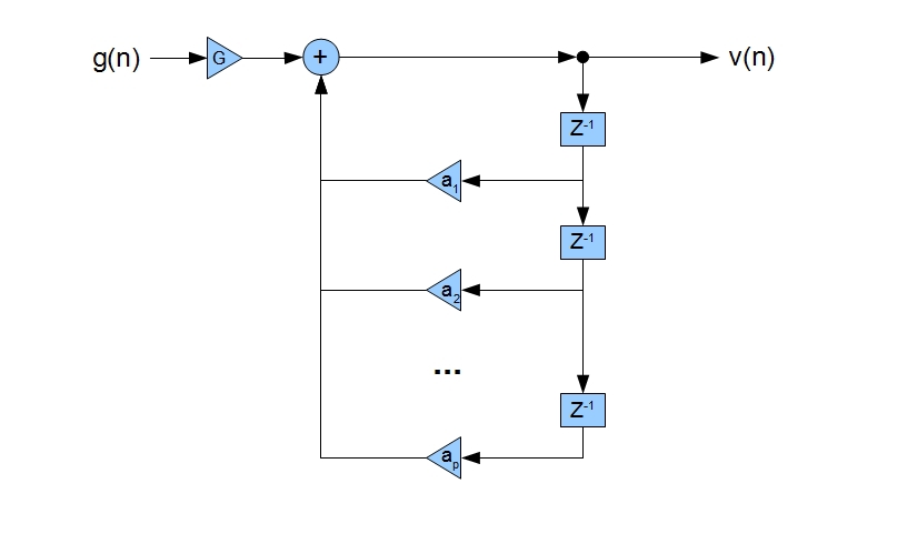
Using the above transfer characteristic of the vocal tract, it can be shown that the signal at the output of the system has the following form in the time domain:



A very interesting result: a complex sound formation process in the vocal tract is reduced to the fact that the signal at the system output at time n is a superposition of the input signal at time n, multiplied by a constant, and a linear combination of the previous output samples at times n - 1, n - 2 ... n - p. But let's not forget that of course this is just an approximation, ignoring many details.

To get a description of the state of the speech path on the analyzed segment of speech, it is necessary to solve the problem of estimating the coefficients a_k and G. The theory of adaptive filtering as a whole, and the LPC model in particular, allow solving this problem relatively simply and computationally efficiently. The resulting description of the vocal tract will be far from exhaustive, but sufficient for many tasks.

Finding LPC Ratios

To solve the problem of estimating the coefficients a_k, it is convenient to introduce the concept of a linear prediction filter, the task of which is to obtain reliable estimates of the desired coefficients (we will further denote the estimates as a'_k). The output of the prediction filter (v '(n)) can be subtracted from the signal at the output of the vocal tract (the resulting difference will be called “signal-error”):



e (n) is a signal-error. The coefficients a'_k, along with G, are called linear prediction coefficients, LPC coefficients. In the case when the estimates a'_k are close to the true values ​​of a_k, e (n) will tend to G ∙ g (n). Note that the linear prediction filter in this problem is the inverse filter to our approximation of the vocal tract. If the estimates a'_k are close to true a_k, then this filter (denoted as v ^ (- 1) _k) is able to reverse the effect of the speech path on the signal g (n) up to a constant G:



Let us return to the estimates a'_k. Choosing a certain segment of the signal for analysis (suppose length M), using the expression (3), we can obtain the error signal vector of a similar length. The question is - how now, having this vector, form well-founded estimates a'_k? This problem can be solved using the method of least squares . To do this, we search for the minimum of the function E_n, the value of which is equal to the average of the sum of the squares of the error signal values ​​on some analyzed time interval (the function E_n is nothing other than the rms error ). In other words, the parameters a'_k are sought for which the root-mean-square error function E_n takes the minimum value. The standard error in our case is expressed by the formula:



Finding the mean implies a division by the number of elements (multiplication by 1 / M), however, this factor will not affect the solution of the desired system, so it can be omitted.

Once again, for clarity, we describe what formula (4) expresses:

1) in the vicinity of the time point 'n', M samples of the signal are taken (usually from n to n + M - 1). The number M depends on the sampling rate of the signal and our assumptions about the stationarity interval of this signal.

2) For the selected samples, an expression is compiled corresponding to the prediction error e (m), m = n: n + M-1

3) The average of the squares e (m) is found (in the expression for the average, we omit the division by the number of terms of the sum).

4) We will minimize the average E_n (which is a function of the reference number n).

Why is the standard error used as a measure of the reliability of our prediction filter? Firstly, it is a good numerical approximation of the variance of a random process in some cases. If we assume that our error is distributed normally and our prediction filter is not very biased, then the root-mean-square error will tend to the dispersion D [e (m)] and we, therefore, look for the minimum dispersion of our error signal. Secondly (although this is probably not the cause, but a convenient consequence), it is very convenient to differentiate this function by the desired a'_k, and it is convenient to find the minimum of the function using differentiation.

Expanding the square sign under the sum in (4) and equating to zero the values ​​of the derivatives of E_n for each a'_k, it is possible to obtain a system of P linear equations of the form:



We will not also give a detailed conclusion (5) from (4) - for this we need to apply several formulas from school algebra and some formulas for converting certain amounts . The system of equations (5) is the “core” in the LPC algorithm. The index i corresponds to the number of the equation in the system (the number a'_k, which took the derivative) and, like the index k, passes all values ​​from 1 to P. Recall that P corresponds to the number of pipes in the model that approximates the voice path. The same number is called the linear prediction order. The solution of systems of linear algebraic equations is a separate applied area with its mathematical apparatus, therefore we will not go deeper into this task. We only say that for solving the system (5) specifically, taking into account its properties, as a rule, Cholesky decomposition or Levinson-Durbin recursion is used.

Having solved the system of P equations from P unknowns, we get the estimates a'_k, and it remains only to find the gain factor G. In the LPC method, the estimate of G is found after the estimate of a'_k, assuming that the signal at the input of the filter V is either offset in time n is a discrete delta function (single impulse at time n), or white noise. In both cases, G can be found from the relationship:



The very derivation of this formula is purely mathematical (that in the case of the delta function, that in the case of white noise) and how to explain the physical meaning of this formula popularly, the author of the article does not represent - let’s leave it as it is. However, the very assumption that the input signal suddenly became a single impulse or white noise should be explained in more detail.

Strictly speaking, at the exit of the glottis in the larynx - at the input of the vocal tract, we have either a “laryngeal” impulse, or a colored noise signal, but not the delta function or white noise. And here, in the theory of LPC, a very tricky “feint with ears” is made. We imagined the larynx as part of the vocal tract and say that it was precisely the larynx that allegedly included either a single impulse or white noise. Thus, the concept of the vocal tract is somewhat broadened within our model, and in order to take into account the new model effects that make a “laryngeal” impulse from a single impulse, and colored noise from white noise, we increase the linear prediction order P. Moreover, we go further and include in our “LPC-filter” effects associated with signal emission, which we also compensate by adding additional coefficients. These operations correspond to an increase in the length of our pole filter, with which we approximate the speech path, which will lead to an increase in the number of its poles, and it is these additional poles that are responsible for the imaginary transformation mentioned above. Obviously, in this case, the LPC model no longer fully corresponds to the initial discrete filter that approximates the speech path. However, ideologically, these two approaches remain very close, if not to say “related”. Using the LPC, it is impossible to reconstruct the g [n] excitation signal of the vocal tract as we would like at the beginning. Nevertheless, the final approximation of the frequency response of the vocal tract (coefficients a'_k), obtained using LPC, is sufficiently accurate for many problems.

Once we talked about choosing the order P, it is logical to give some general recommendations on his choice. It is believed that, on average, formant frequencies in a speech signal are located with a density of approximately 1 formant per kilohertz. Then, since each complex pole of our model filter corresponds to one formant frequency, it is convenient to choose an order like:



where [] is the rounding to the nearest integer, Fs is the sampling rate of the signal in hertz. To compensate for the effect of combining the larynx and the vocal tract, as well as to take into account the effect of the radiation of the signal by the lips / nose in the model, various sources recommend increasing P by an additional 2–4 coefficients.That is, for operation, for example, with a 10 KHz signal, the order P can be chosen equal to 12-14 coefficients. Some authors also advise to use the density of "1 formant at 1200-1300 Hz" when analyzing a female voice. This is due to the shorter length of the vocal tract in women and, as a consequence, the higher formant frequencies in female voices.

LPC summary

What ultimately gives us the calculation of the LPC coefficients for a certain signal:

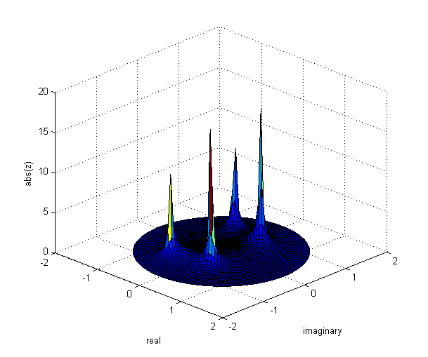
1) The output of the LPC calculation algorithm is a set of numerical coefficients that describe the pole filter. These coefficients in their pure form allow us to obtain an expression for the output of a given filter in the time domain (expression (2)), as well as a general view of its z-characteristics (expression (1)). Since this filter is polar, it is based on recursion and it is not possible to express the impulse response for such a filter. Using the z-characteristics, however, a full analysis of the resulting filter is possible in both the time and frequency domains.

2) z-, , . . ( , LPC — P, M, n. .)

3) LPC - ( , ) , -. ( )

Below, for example, is the logarithmic spectrum of a signal obtained by a conventional FFT and using LPC. Processed vowel "A", pronounced in a male voice.



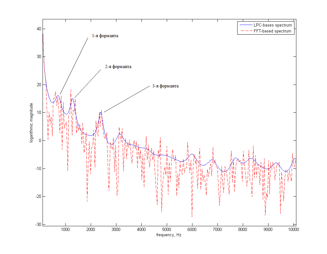
As you can see, the “LPC spectrum” is some smoothed version of the usual “FFT spectrum”. At the same time, formant frequencies appear as “bright” local maxima, which is a good “start” for their detection and tracking.

LPC application for speech path analysis

, , , . r_k, k – . . ( ) , , . , , , (1), LPC-.

- LPC- – «» . , , LPC- , - ? 100% . , LPC- r_k, – r_k a'_k. PARCOR (partial correlation) . . . LPC- PARCOR-, r_k. : LPC , , ( P). , - , LPC- , LPC. , , — , . . . , , .

There are many works whose authors solve the problem of restoring the function of the area of ​​the vocal tract, and in these works the LPC coefficients take not the last place in the mathematical tools used. In particular, LPC is often used as a basic method for determining the values ​​of formant frequencies, with the help of which the function of the vocal tract area is already restored.

LPC , , , — . , , , LPC, - .

findings

LPC- . , , . :

—

—

— ( )

HPN- (Harmonics-plus-noise) , .

:
[1] JL Flanagan. Speech Analysis, Synthesis and Perception.
[2] LR Rabiner, RW Schafer, Digital Processing of Speech Signals // ( )
[3] .. , 2- // ( , «» , )
[4] Mark Hasegawa-Johnson, Lecture Notes in Speech Production, Speech Coding, and Speech Recognition
[5] G. Fant. Speech Acoustics and Phonetics. Selected Writings .