Sinusoidal modeling and typographical errors in Caltech

This post is about a relatively new method of signal processing, described in the article Adaptive data analysis via sparse time-frequency representation , as well as about a tiny, but confusing me personally, error. This article was published in 2011 by Professor of Applied Mathematics at the California Institute of Technology, Thomas I. Hou and Shi Zoqiang, and, probably, by the time you read it, they had already corrected it.
I stumbled upon this article in the search for various methods of time-frequency analysis of nonlinear and non-stationary signals - in my case, ultrasound signals from moving formed blood elements in human vessels. The essence of this analysis is to track changes in the signal characteristics, in other words, we want to know the dependence of the frequency components of the signal on time. With the exception of the widely used methods - spectral and wavelet analysis, such methods as EMD (empirical mode decomposition) and sinusoidal modeling were found, which will be discussed further here.
The empirical mode method is fairly simple to use, but is not particularly developed in terms of the validity of the results obtained. Thomas Hou and Shi Zoqiang went further in the development of the mathematical apparatus and proposed their own method of sinusoidal signal modeling. His idea is sparse decomposition of a harmonic signal with smooth amplitudes. What result we expect to get - in the picture above. In this case, the signal received by the function f (t) = 6t + cos (8πt) + 0.5 cos (40πt) was decomposed. The decomposition of the signal, of course, is not unique; therefore, the criterion of the minimum harmonic components was introduced, and the problem was formed as follows:


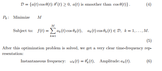
The solution of the P0 problem will be harmonics with amplitudes a and phase theta functions, whose derivatives will correspond to the signal frequencies. The authors propose to solve this problem recursively: extract one harmonic component, get the remainder (median) - work with it, extract the next harmonic from it, get the remainder, and so on. Since the median should be much smoother than the signal, finding the harmonic boils down to solving the following problem:

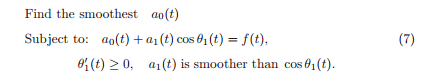
where a1 * cos (theta1 (t)) is the resulting harmonic, a0 is the median. The smoothness of the amplitude is determined by the total variation:


The greater the smoothness of the function g, the closer to zero its (n + 1) derivative, the lower the total variation of the nth order, respectively. One can say more: the smaller the order of the polynomial with which we can interpolate, the smoother the function. It is logical to assume that it would be best to look for a minimum of zero order variation, however, in this case we risk getting a piecewise constant function (staircase effect) and losing some of the higher order information we need (for example, curvature). The authors of the article propose to reduce the variation of the third order, directing the fourth derivatives to zero, thereby making something similar to approximation by cubic splines. As a result, we are looking for min TV ^ 3 (a0). But it is also important for us that a1 is sufficiently smooth, so at best we have to find min TV ^ 3 (a0) + min λ * TV ^ 3 (a1), where λ is the Lagrange multiplier, which in this case plays the role of the weighting factor . For simplicity, the authors left λ = 1 and arrived at the following problem:
')

Algorithm

To solve this problem, an iterative algorithm is proposed. One more harmonic is added to the condition - b1 * sin (theta1 (t)), its smoothness also becomes our goal. Initialize the phase function theta ^ 0 so that it is an increasing function that satisfies the condition cos (theta ^ 0) = f (t), and run the main iteration:

In the first step, we minimize the total amplitude variations. On the following - we update theta using the above formula, then check how much it has changed. By the end of the algorithm, it is assumed that the amplitude b1 will be already negligible, respectively, the artcg (b1 / a1) will be small, and theta will converge to some value. This will be our phase function. Having received theta ^ n, we select the first harmonic a1 * cos (theta1 (t)), where theta1 = theta ^ n. Then we run this algorithm on the remainder, that is, we work with the values ​​f (t) = a0 + b1 * sin (theta1 (t)). Select the next harmonic a2 * cos (theta2 (t)), continue with the remainder. And so on until the norm of the residue is negligible. I took the first norm. For those who do not remember its definition:


To apply the problem of finding the minimum of the general variation, the authors reduced to the L1-minimization problem, replacing the differential equation with the difference one. We have a signal, or rather an ordered set of N points (nodes), which we want to expand, that is, to represent as the sum of the vectors a0, a1 * cos (theta1 (t)) and b1 * sin (theta1 (t)). And in the reformulated problem an unfortunate typo was noticed:

Assuming that a0 ^ n, a1 ^ n, b1 ^ n are grid functions, we approximate their fourth derivatives by multiplying them by the matrix D ^ 4. Then, minimizing the sum of the moduli of the obtained values, we reduce the corresponding variations. Everything is logical and plausible, but, having implemented this algorithm, I was horrified to see the results - it turned out something completely chaotic. Long trying to detect an error in the code, I finally realized that the error was in the article.
The fact is that by multiplying Phi by x, we get a vector, where the elements are the sums of the derivatives a0 ^ n, a1 ^ n, b1 ^ n at the corresponding points. That is, we minimize the total variation from (a0 ^ n + a1 ^ n + b1 ^ n), rather than the sum of the three variations, as indicated above.
Error is an error, found, corrected and forgotten for several months. And so, on the May holidays, I was still torn to write a letter to professors with the proposal to replace the article min || Phi * x || at min || D ^ 4 * a0 ^ n || + || D ^ 4 * a1 ^ n || + || D ^ 4 * b1 ^ n ||. Surprisingly, an hour later, an answer came from Professor Hou with the phrase “Thanks for your email. We will study your note and get back to you soon ”and a simple“ Tom ”signature.

After another 6 hours, a letter came from Professor Shi:

Dear Aleksandr,

Thanks a lot for your email. We did make a typo here.
\ Phi should be diag (D4, D4, D4)
algorithm. Thanks.

Best,
Zuoqiang shi

Naturally, my amendment and what they wanted to write are identical. The only thing I must note is that if you do not store the matrix Phi under the assumption that it is sparse, that is, to store a bunch of zero elements, the memory may soon end.

How the L1-minimization problem is solved

For their algorithm, professors propose the Bregman iteration and L1-regularized least square method split methods. However, these methods are quite fresh and, probably, not all packages are sewn up. Who is lazy (like me) to implement any of the algorithms for finding the minimum of the first norm, it will be useful for him to find out how this problem reduces to the more common linear programming problem. The original task is as follows:


provided

where A is the NxM matrix, Phi is the KxM matrix, x is a vector of dimension M.

It is equivalent to the following linear programming problem:


under conditions



where phi (i, j) are elements of the matrix Phi.

Formally, the transition can be done as follows. To the vector x is added K variables, thus it becomes the dimension of K + M:

To matrix A is added a zero matrix of NxK dimension:


The vector c (coefficients in the LP problem) consists of M zeros and K units:


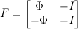
The matrix F is composed of the matrix Phi and the unit matrix I. The dimension F - (2 * K) x (M + K):



Thus, a formalized task looks like this:

under conditions

results

Here are the results of the algorithm for the previously mentioned example f (t) = 6t + cos (8πt) + 0.5 cos (40πt). On the graphs, the values ​​obtained by this algorithm (blue) are compared with the analytical values ​​(red) and the values ​​obtained by decomposition into empirical modes (black).

The following example shows how this method helps to track frequency variations of a signal.



The article contains other examples, as well as the results of the algorithm on real data.

Total

The algorithm is very interesting and, in my opinion, requires further analysis, the benefit of space for thought is full here. Its obvious disadvantages are high computational complexity, as well as sensitivity to noise and, as a result, unstable operation with noisy data. The authors propose to solve the problem of sensitivity using low-pass filtering and Fourier transform. But more about that another time.
Finally, I want to once again boast and say that, apparently, it happens that professors in Caltech make, however small, mistakes, but a Russian student, who does not have a bachelor so far, can point this out to them.