Spy on the throwing of the neural network

In the comments to my previous article about what is happening in the neural network, the phrase slipped that, unfortunately, the visualization of learning processes is rarely possible on real tasks with big data. Really so sorry. Let's try to fix it. Under the cat, I propose a simple and, surprisingly, informative visualization of the learning process of a neural network that does not depend on the nature of the task, nor on the properties of the network itself, that is, available for an arbitrarily complex task.

Training

')
The problem to solve the network is taken from the previous article. The neural network receives two numbers at the input - two coordinates, and it is proposed to determine whether this point is above the graph. At the output is expected to be -1, +1 or 0 (if the point exactly lies on the graph). This time the task will be symmetrized. Coordinates are taken from the range [-0.5; +0.5], the point 0.0 will be exactly in the center of the picture and the graph also passes through it, so the expected value at this point is also 0. The area above the graph and the area under the graph are equal. So, on average, we have 0 at each input, and 0 is also expected at the output on average.

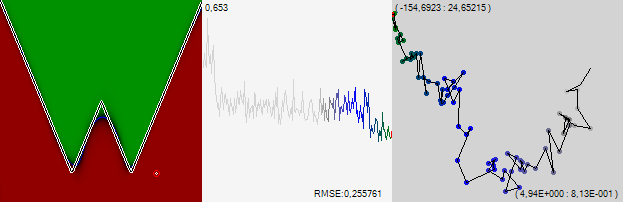
We will take a network consisting of 3 layers with 15 neurons in each (the activation function is hypertangent) and we will train it using the classical back propagation method and stochastic gradient descent with a gradually slowing rate. We will see what the network has learned, as shown in the image above. Networks will be offered all points of the range, and depending on the response, the point will be painted in different shades of green (if the network’s response is greater than 0), shades of red (if the value is less than 0), and finally, shades of blue (if the answer given by the network is 0 or its neighborhood). The picture above shows the results of a fully trained network, with a root-mean-square error of 0.22, if you look only at the sign of the correct answers, it will be much more than 99%

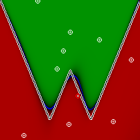
I note, by the way, that a very ordinary neural network simply cannot cope with this seemingly simple task. It always turns out something like this:



To solve this problem, we, as suggested in the last article, will make three inputs to the network and give the constant 1 to the third. After that, the problem becomes feasible for the network.

All code for testing and independent experiments can be viewed in the previous article.

Visualization

Now the main idea of ​​visualization. So, we have a network with a total of 510 synapses. The process of learning this network is a change in the weights of these synapses. This can be represented as a walk through 510-dimensional space. And at every point in this space, the network has some kind of efficiency. This effectiveness forms a relief. Just like in the picture, only not a 2-dimensional picture, but a 510-dimensional one. While it is difficult to imagine, I agree. But this is a relief, which means that the network traveling along this relief will behave in approximately the same way as we when we are looking for a road by touch. The human brain is adapted to solve such problems, which means that the behavior of the network may be intuitive to us.

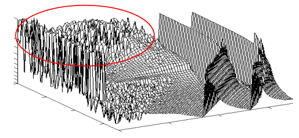
There are areas where the relief is smooth, but mostly it is strongly cut, as in a circle circled area. However, even if the terrain is very toothy and consists of a large number of local maxima, it can have a fairly smooth envelope.

The learning algorithm, getting shocks from individual training examples, can skip the teeth of this graph, but in general it will crawl down. Looking at this movement, we will see that the point in the 510-dimensional space is torn, but on average it crawls more or less in one direction. Let's follow these movements.

Of course, not everyone can trace the motion of a point directly in 510-dimensional space, so we will cheat. We arbitrarily project this 510 dimensional space onto the two dimensional screen space. Each synapse is assigned a random unit vector modulo, and we will summarize all these vectors multiplied by the synapse weight. According to the law of large numbers, the sum will be close to point 0. To begin with, we take a random untrained network and see what the trajectory will look like if we mark a point after each individual learning example.



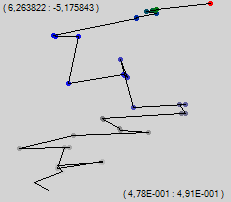
The numbers in the upper left corner are the position in the space of the upper left corner of the picture, and the numbers in the lower right are the dimensions of the imaged area.

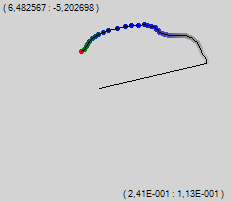
We see the "Brownian" movement, which traces the general trend upwards. Let's change the algorithm on the go. We will use the same reverse error propagation, only the training change will not be applied all at once, but gradually, over several steps. In my program, I call this method "gradient descent of slow learning." At the same learning rate, we get another 35 points.



We see that this algorithm has a much greater smoothness. Let's dock a few more dozens of points and with a larger magnification we will see how the network crawls through space, looking for a path in the smoothed relief.



It is immediately clear why the second algorithm is less prone to random losses of the minima found. It is interesting that in some areas the network creeps gradually, and in some it changes direction as if it was received on the forehead. It is interesting to see how these points differ.



In the first picture, we see that the network is slowly but surely crawling in one direction. New points fall into the area where the network already receives the correct answer. In addition, it is a pure green area in which the value at the output of the network depends little on the input data. The derivative of the error is small, and accordingly the control action on the network is small. But in the second picture, the next point falls close to zero, where the network has a large value of the derivative of the error. In addition, the point is below the graph, the value -1 is expected there, and the network showed green there, judging by the color, approximately +0.8. A very big mistake coincided with a large derivative, the network got a kick from below and went a new way, upwards. In the last (third) picture, it is clear that the entire blue area has shifted higher. The fact that the direction of movement of the network along the learning path and the direction of the shift of the picture coincided, of course, by chance, but beautiful.

Let the program show not 50 points, but 200, and admire the network learning path. The relief over the 510-dimensional space is not visible to us, but in a blind network crawling along the invisible labyrinth, problem areas are clearly guessed - invisible walls, which the network knocks here and there, and crawls in a new direction.



We see that after only 200 educational examples, the left edge of our dividing blue line began to gradually curl upwards. Let us return to the classical back-propagation algorithm of the error (“jerky”) and add another 200 points.



We see, despite the fact that the network began to twitch like crazy, it continued to move, in principle, in the same direction and, in principle, with the same final speed. You can quite vividly imagine that canyon, in which the network crawls to a better life, feeling the walls. Despite its 510-dimensional, the relief is quite well traced. And in the picture, not only the left but also the right edge of the chart began to bend upwards.

Why do we see this monotonous movement? It is clear that the network will learn until the edges of the blue line look cool up on both sides. To do this, the scales of some synapses will need to change a lot, to become much more than now. Some examples only slightly shift them, and it will take a lot of examples before they acquire their great values. It is the gradual increase in the weight of such synapses that pulls the trajectory of the network training along a well-marked trend in the direction that we assigned to this synapse at the very beginning. Synapses, the values ​​of which in the process of learning vary in a narrow range, are hardly noticeable on the trajectory.

So what do we understand?

Relief can not be seen, at least it is difficult to do on a home computer, but by the behavior of the network, you can understand what it is.

Add gas

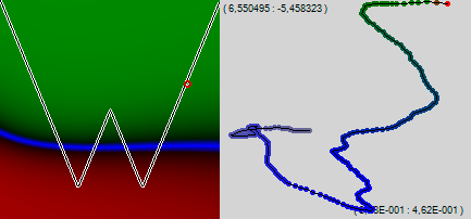
Let's continue to train the network, but to draw every next point on the learning path, not after every single learning example, but after 1000.



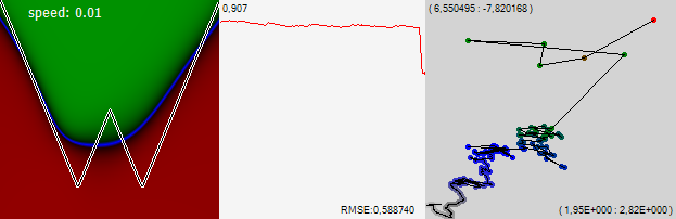
It is seen that the network as a whole continued to crawl up and to the right, bending the edges of the graph upwards. The graph in the middle of the figure is the standard error for the last 1000 examples. One point on this graph corresponds to one point on the learning path on the right picture. It is clearly seen how the error began to decline sharply when we increased our pace. The number in the upper left corner of the graph is the scale in which the graph is displayed, and the error value itself is displayed in the lower right corner.

So, we will continue our journey through a very multidimensional space.



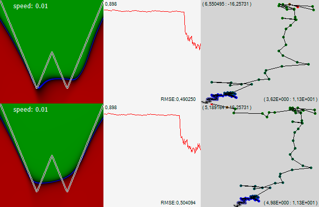
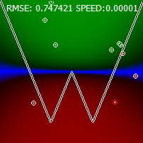
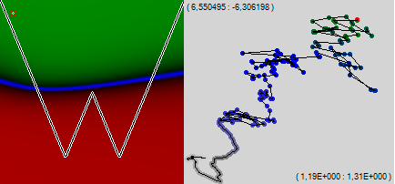
Note! At some point, the network ceased to drift monotonously in one direction and read out in one area. But then another sharp movement pushed the net out of this improvised lake, and it went quite quickly to the left. The graph of the error shows that on this part of the trajectory the error was slightly less. But obviously not enough to make any decisions. And, meanwhile, looking at the left picture, you can see that in this lake the network has learned to understand that the graph, which it studies two minima. After, having broken the net to the left, this knowledge has lost. Let's agree that the next time, when the network ceases to drift monotonously and begins to more carefully touch one interesting place, we assume that it has found something useful, and reduce its speed, giving it the opportunity to study the found place more closely.



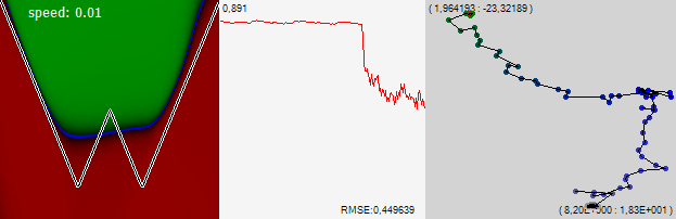
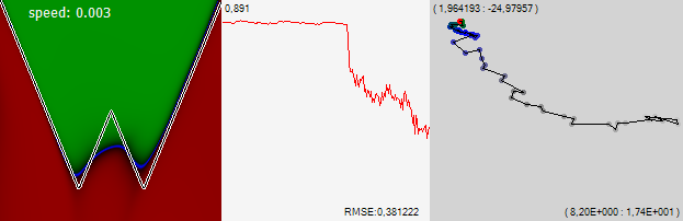
And now the network again begins to carefully examine the new good place. We like it, we reduce the speed by 3 times. As we see, for our vision we were rewarded with a dramatic improvement in error, and the network began to look for a new solution for itself already in a limited area of ​​space, in which, apparently, there is a good local minimum.



To consolidate the priority I will call it with my name: “visualization kraidiky”, until someone came up with a less euphonious and individuality name for it.

So, what are our conclusions?

1. Observing the trajectory of learning network, you can clearly distinguish when the network is located in a connected compact area of ​​local minima, and when moving along a gradient along a canyon or slope from one area to another. Probably, having observed the network, one can discern other features of the invisible terrain over which the network travels.
2. The difference is so noticeable that it can be used to make decisions about changing the training mode of the network. Changes in the mean-square error associated with these features of the relief are also observed, but they are very minor, difficult to distinguish against the background of noise and cannot, in all likelihood, serve as the basis for decision-making. Sometimes you can even see the areas where the network error is growing. But visualizations of both types show that the network goes in the chosen direction, and there it finds much better solutions, the effect of which will become noticeable later, like, for example, two minima in our problem.
3. My algorithm is as follows: if the network ceases to go along the canyon and begins to study a limited area, then you need to see if there are good, much better solutions than those encountered on the way to this area. If yes, then reduce the speed, allowing the network to more closely examine this area, and, perhaps, find a good solution for it. If good solutions are not found, then you can wait until the network itself leaves the area and leaves it by some canyon, or, if the search is delayed, push it out, increasing the speed.
4. The method of visualization of the network learning process described in the article is unexpectedly informative. Obviously more than the observation of the average error, and sometimes even more than comparing the obtained knowledge map with the original problem.
5. The way of visualization does not depend in any way on the nature of the task, nor on the network topology, it can be used to visualize the learning process, including complexly organized networks, with difficult tasks that are poorly amenable to visualization.

In conclusion, I suggest you enjoy the spectacle of the learning network. At 1:26, I can see how the area of ​​minima found by the network did not suit me, and I sent it to look for another one, just by adding learning speed.


UPD: Visualization has one drawback. All synapses are considered as equal in importance. While in reality this is certainly not the case. Some synapses have a very strong effect on the final result, some almost no role play. It would be nice to multiply the significance. A good measure of significance is the derivative of the error by the weight of a given synapse. But the problem is that for different learning examples it varies greatly. It would be necessary to average over the entire training sample, but in my task the training sample is different each time and the importance walks too much and jams the picture even if it is averaged over the last 1000 training examples. Poca has not figured out how to solve this problem.

UPD 2: Solved the problem. I take the rms derivative for all the time of training. On hundreds of thousands of examples, the significance of synapses becomes stable and differs by almost three orders of magnitude for different synapses. However, it is not strange, such visualization is less informative. Or informative in another way, I do not even know how to say it.



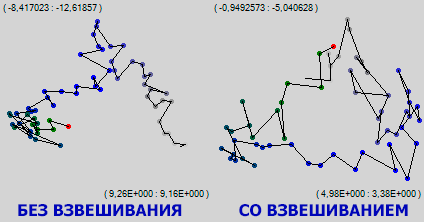
The picture shows the same part of the network training. It can be seen that, where simple visualization showed an area of ​​local minima, in which the network had been hanging around for a long time, weighted visualization of trampling in one place did not record, moreover, steady drift up and to the right is noticeable on the green part of the trajectory. Apparently, while the network as a whole is marking time in one small area, it moves very intensively and meaningfully with its best synapses. As they say, at the cellular level, I am very busy.