Creating a robot balancer on arduino
For a long time, I was haunted by the desire to calculate some rather complicated mechanism and implement his life.
The choice fell on the reverse pendulum problem. The result on the video:
I will not give the derivation of the equations of motion, after all, this is the third year of the institute. For those who are interested in the conclusion, at the end of the article there is a link where it is described in more detail.
We will present the system as follows:
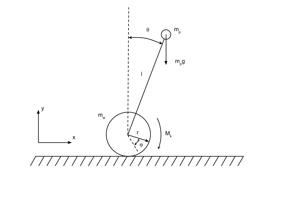
A pendulum is a mass m p attached at the end of a weightless rod of length l. At the other end of the rod, an engine is attached that develops the maximum moment M k and transmits it to a wheel of mass m w and radius r.
The control task is to stabilize the pendulum in a vertical position and return the wheel to the initial position.
')
The equations of motion describing the inverse pendulum can be represented as follows:
They seem rather unpleasant, but the robot itself knows nothing about them, and the control uses a linearized model, that is, this:
I envy people who have a PID controller. I spent several hours adjusting its coefficients, but failed to achieve a worthwhile result. The supervisor advised to use a linear-quadratic regulator ( wiki ). This regulator, unlike the PID controller, is simply the product of its coefficients and errors for each coordinate. No discrete analogs of the derivative and the integral. However, to calculate it, one needs a system model and the ability to solve the Riccati equation, or Matlab.
In the matlab, the regulator's calculation is such a set of commands:
Here the matrices A and B are the corresponding matrices from the linearized model with the substituted values of the real robot.
The Q matrix determines how much you need to penalize the system for deviating from the origin, note, in our case, the coordinates include speeds.
The matrix R determines how much it is necessary to penalize the system for waste of energy by control.
The variable K will be the coefficients of the regulator.
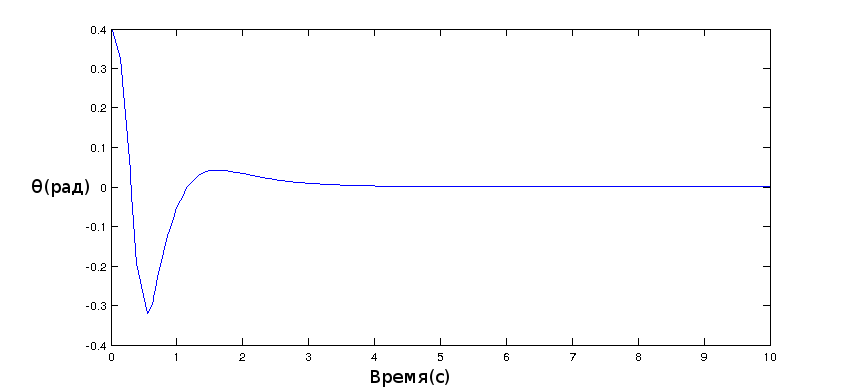
In Matlab simulink, you can easily emulate a system if someone needs a link to a repository with a mathematical model at the end of the article. Here I will only bring graphics.
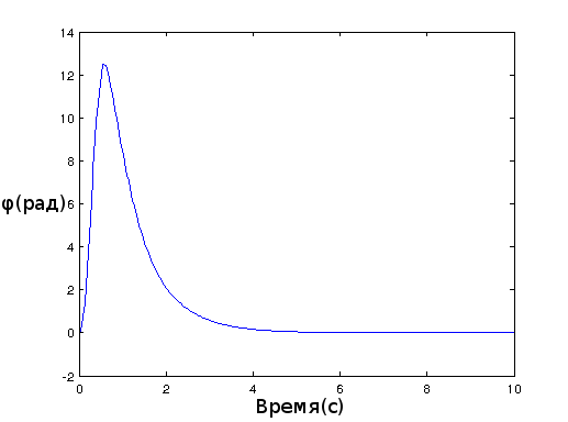
The angle of deflection of the pendulum:
Wheel deflection:
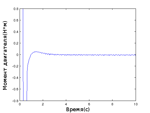
Engine torque:
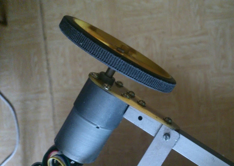
The frame of the robot itself is aluminum profiles 12mm and 14mm, they come into each other. Riveted. Electronics is attached to a piece of fiberglass in the shape of the letter T. Motors are also attached through a glass-fiber laminate adapter.
Initially, I tried to use these motors:
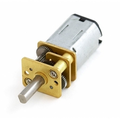
Their torque is 2.2 kg * cm or 0.2 Nm. Based on the simulation, we need much more, so other motors were chosen:
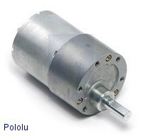
reference to the manufacturer
Maximum torque 14kg * cm or 1.4Nm. They consume up to 5A of current, so the popular L293D among arduinschikov here will not work.
To determine the angle and angular velocity is used IMU - gyro and accelerometer. I had a board with a L3G gyroscope and an accelerometer with an LSM303 magnetometer. There are a lot of similar boards and I will not give a code for obtaining sensor values. However, the sensor readings need to be filtered, as the gyroscope constantly goes away, and the accelerometer is noisy and strongly lying, if the robot starts moving without changing the angle.
Different filters are used, but the Kalman filter and the RC filter (complementary filter) are most popular. I use this code:
Works not perfect, but good enough for this task.
The next sensor is a quadrature encoder on a motor. It generates rectangular pulses on 2 of its findings:
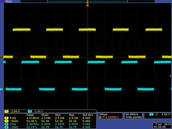
You can read them either by interrupts or by reading values in a loop. On arduino playground there is a wonderful article with code examples.
It remains to obtain the angular velocity of the wheel. Here comes the school formula for the distance traveled / elapsed time.
ToPhiRad translates the number of encoder ticks into a wheel angle, my encoder gives out about 2240 ticks per rotation. To get the angle you need to multiply the ticks by 2 Pi and divide them by the number at full turn of the wheel.
Sensor readings go to the LQR controller:
The coefficients are taken from Matlab, although for better stability I corrected the first 2 coefficients.
My driver, or rather his library, takes values from -400 to 400. I assumed that at 400 he gives 12V to the motor, i.e. the motor develops the maximum torque (1.4 Nm). Dividing 400 by 1.4, we get the conversion factor from Nm, which LQR produces, to values that the driver understands.
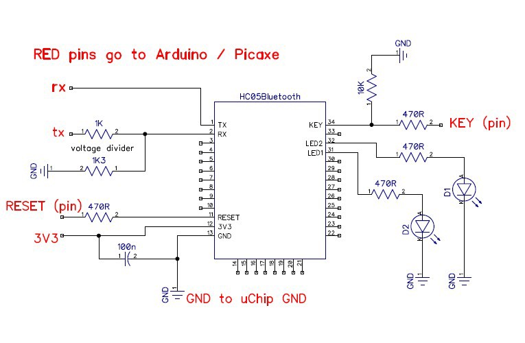
Just stabilizing the robot at one point is not very interesting, so the BT-module HC-05 was added to it. The module connects to the serial port of the microcontroller. It works at 3.3V, and arduino at 5V, so you need to connect the receiving input module through a voltage divider. Here is the connection diagram:
During the cycle, the microcontroller polls the module for symbols:
In the end, the readings of the sensors go to the regulator, and its control and user action go to the motors:
Once every 50 milliseconds, the telemetry angle of the robot is sent:
We will manage from the phone under android.
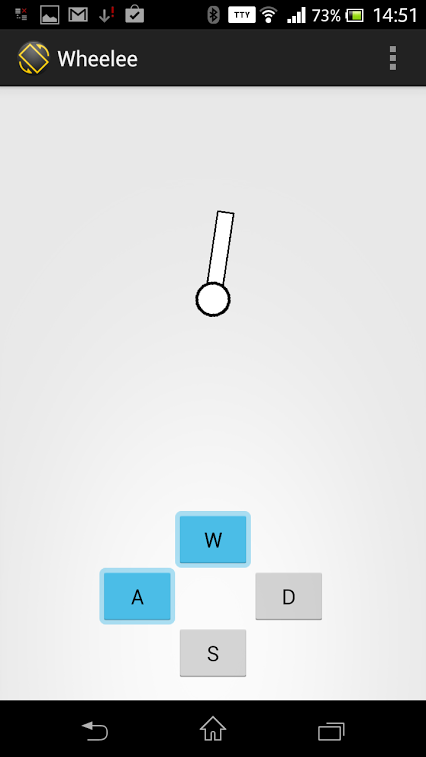
When launching the application, we ask the user to choose who to connect to, the bt-module should already be paired with the phone (standard code 1234).
After selecting the device, connect to it:
After connection, a stream starts, which communicates between the application and the robot:
A thread sends a message to the main application thread via a Handler, which is defined like this:
balancerView is a descendant of the SurfaceView class, it deals with displaying the current position of the robot.
Here is his redrawing method:
Commands are sent to the robot when onTouch events appear, so that you can control the robot while holding the button.
The most pleasant thing about the whole building is that the mathematical model converges with the physical implementation. The construction of the piece of iron does not present itself in itself, but the selection of the correct motors, the height of the robot, the mass of the load from above and the synthesizing of the control is a rather interesting task.
As promised, the derivation of the equations of motion of the inverted pendulum on the wheel: The derivation of equations and a little about the construction
repository on github
The choice fell on the reverse pendulum problem. The result on the video:
Mathematical model
I will not give the derivation of the equations of motion, after all, this is the third year of the institute. For those who are interested in the conclusion, at the end of the article there is a link where it is described in more detail.
We will present the system as follows:
A pendulum is a mass m p attached at the end of a weightless rod of length l. At the other end of the rod, an engine is attached that develops the maximum moment M k and transmits it to a wheel of mass m w and radius r.
The control task is to stabilize the pendulum in a vertical position and return the wheel to the initial position.
')
The equations of motion describing the inverse pendulum can be represented as follows:
They seem rather unpleasant, but the robot itself knows nothing about them, and the control uses a linearized model, that is, this:
Control synthesis
I envy people who have a PID controller. I spent several hours adjusting its coefficients, but failed to achieve a worthwhile result. The supervisor advised to use a linear-quadratic regulator ( wiki ). This regulator, unlike the PID controller, is simply the product of its coefficients and errors for each coordinate. No discrete analogs of the derivative and the integral. However, to calculate it, one needs a system model and the ability to solve the Riccati equation, or Matlab.
In the matlab, the regulator's calculation is such a set of commands:
A=[0 1.0 0 0;0 0 -140 0;0 0 0 1.0;0 0 28 0] B=[0;212.85;0;-19.15] Q=[5 0 0 0;0 5 0 0;0 0 1 0;0 0 0 1] R=1500 [K,S,e]=lqr(A,B,Q,R) Here the matrices A and B are the corresponding matrices from the linearized model with the substituted values of the real robot.
The Q matrix determines how much you need to penalize the system for deviating from the origin, note, in our case, the coordinates include speeds.
The matrix R determines how much it is necessary to penalize the system for waste of energy by control.
The variable K will be the coefficients of the regulator.
Simulation
In Matlab simulink, you can easily emulate a system if someone needs a link to a repository with a mathematical model at the end of the article. Here I will only bring graphics.
The angle of deflection of the pendulum:
Wheel deflection:
Engine torque:
Implementation in the gland
The frame of the robot itself is aluminum profiles 12mm and 14mm, they come into each other. Riveted. Electronics is attached to a piece of fiberglass in the shape of the letter T. Motors are also attached through a glass-fiber laminate adapter.
Initially, I tried to use these motors:
Their torque is 2.2 kg * cm or 0.2 Nm. Based on the simulation, we need much more, so other motors were chosen:
reference to the manufacturer
Maximum torque 14kg * cm or 1.4Nm. They consume up to 5A of current, so the popular L293D among arduinschikov here will not work.
To determine the angle and angular velocity is used IMU - gyro and accelerometer. I had a board with a L3G gyroscope and an accelerometer with an LSM303 magnetometer. There are a lot of similar boards and I will not give a code for obtaining sensor values. However, the sensor readings need to be filtered, as the gyroscope constantly goes away, and the accelerometer is noisy and strongly lying, if the robot starts moving without changing the angle.
Different filters are used, but the Kalman filter and the RC filter (complementary filter) are most popular. I use this code:
float lastCompTime=0; float filterAngle=1.50; float dt=0.005; float comp_filter(float newAngle, float newRate) { dt=(millis()-lastCompTime)/1000.0; float filterTerm0; float filterTerm1; float filterTerm2; float timeConstant; timeConstant=0.5; filterTerm0 = (newAngle - filterAngle) * timeConstant * timeConstant; filterTerm2 += filterTerm0 * dt; filterTerm1 = filterTerm2 + ((newAngle - filterAngle) * 2 * timeConstant) + newRate; filterAngle = (filterTerm1 * dt) + filterAngle; lastCompTime=millis(); return filterAngle; } Works not perfect, but good enough for this task.
The next sensor is a quadrature encoder on a motor. It generates rectangular pulses on 2 of its findings:
You can read them either by interrupts or by reading values in a loop. On arduino playground there is a wonderful article with code examples.
It remains to obtain the angular velocity of the wheel. Here comes the school formula for the distance traveled / elapsed time.
#define ToPhiRad(x) ((x)*0.00280357142) timer_old = timer; timer=millis(); G_Dt = (timer-timer_old)/1000.0; dPhi=(ToPhiRad(encoder0Pos)-lastPhi)/G_Dt; ToPhiRad translates the number of encoder ticks into a wheel angle, my encoder gives out about 2240 ticks per rotation. To get the angle you need to multiply the ticks by 2 Pi and divide them by the number at full turn of the wheel.
Sensor readings go to the LQR controller:
float K1=0.1,K2=0.29,K3=6.5,K4=1.12; long getLQRSpeed(float phi,float dphi,float angle,float dangle){ return constrain((phi*K1+dphi*K2+K3*angle+dangle*K4)*285,-400,400); } The coefficients are taken from Matlab, although for better stability I corrected the first 2 coefficients.
My driver, or rather his library, takes values from -400 to 400. I assumed that at 400 he gives 12V to the motor, i.e. the motor develops the maximum torque (1.4 Nm). Dividing 400 by 1.4, we get the conversion factor from Nm, which LQR produces, to values that the driver understands.
Just stabilizing the robot at one point is not very interesting, so the BT-module HC-05 was added to it. The module connects to the serial port of the microcontroller. It works at 3.3V, and arduino at 5V, so you need to connect the receiving input module through a voltage divider. Here is the connection diagram:
During the cycle, the microcontroller polls the module for symbols:
float phiDif=0.f; float factorDif=0.f; float getPhiAdding(float dif){ // - if(dif<200 && dif>-200){return 0.f;} float ret = dif*0.08; return ret; } float getFactorAdding(float dif){// if(dif<200 && dif>-200){return 0.f;} float ret = dif/500*20; return ret; } //======== if (Serial.available()){ BluetoothData=Serial.read(); if(BluetoothData=='w'){ phiDif=200; } else if(BluetoothData=='s'){ phiDif=-200; } else if(BluetoothData=='a'){ factorDif=200; } else if(BluetoothData=='d'){ factorDif=-200; } else if(BluetoothData=='c'){ factorDif=0; phiDif=0; } } In the end, the readings of the sensors go to the regulator, and its control and user action go to the motors:
encoder0Pos+=getPhiAdding(phiDif); lastPhi=ToPhiRad(encoder0Pos); spd=getLQRSpeed(ToPhiRad(encoder0Pos),dPhi,balanceAt-angle,gyroRate[coordY]); float factorL=getFactorAdding(factorDif); md.setSpeeds(spd-factorL,spd+factorL); Once every 50 milliseconds, the telemetry angle of the robot is sent:
if(millis()%50==0){ Serial.println(angle); } Add radio control
We will manage from the phone under android.
When launching the application, we ask the user to choose who to connect to, the bt-module should already be paired with the phone (standard code 1234).
BluetoothAdapter bluetooth; String []boundedItems; protected static final int RECIEVE_MESSAGE = 1; @Override protected void onCreate(Bundle savedInstanceState) { //... bluetooth = BluetoothAdapter.getDefaultAdapter(); if(bluetooth != null){ if (!bluetooth.isEnabled()) { bluetooth.enable(); } } Set<BluetoothDevice> bounded=bluetooth.getBondedDevices(); boundedItems=new String[bounded.size()]; int i=0; for (BluetoothDevice bluetoothDevice : bounded) { boundedItems[i++]=bluetoothDevice.getName(); } showListDialog(); //... } public void showListDialog(){ AlertDialog.Builder builder = new AlertDialog.Builder(this); builder.setTitle("Pick a device"); builder.setItems(boundedItems, new DialogInterface.OnClickListener() { public void onClick(DialogInterface dialog, int item) { connectTo(item); } }); AlertDialog alert = builder.create(); alert.show(); } After selecting the device, connect to it:
private static final UUID MY_UUID = UUID.fromString("00001101-0000-1000-8000-00805F9B34FB"); BluetoothSocket btSocket; public void connectTo(int id){ Set<BluetoothDevice> bounded=bluetooth.getBondedDevices(); for (BluetoothDevice bluetoothDevice : bounded) { if(bluetoothDevice.getName().equalsIgnoreCase(boundedItems[id])){ try { btSocket=bluetoothDevice.createRfcommSocketToServiceRecord(MY_UUID); btSocket.connect(); ct=new ConnectionThread(btSocket); ct.start(); } catch (IOException e) { e.printStackTrace(); try { btSocket.close(); } catch (IOException e1) { e1.printStackTrace(); } showListDialog(); } return; } } } After connection, a stream starts, which communicates between the application and the robot:
private class ConnectionThread extends Thread{ private final InputStream mmInStream; private final BufferedReader br; private final OutputStream mmOutStream; public ConnectionThread(BluetoothSocket socket) throws IOException { mmInStream = socket.getInputStream(); br=new BufferedReader(new InputStreamReader(mmInStream)); mmOutStream = socket.getOutputStream(); } public void run() { while (true) { try { String line=br.readLine(); h.obtainMessage(RECIEVE_MESSAGE, line).sendToTarget(); } catch (IOException e) { e.printStackTrace(); } } } public void sendCmd(char cmd){ try{ mmOutStream.write(cmd); }catch (IOException e) { e.printStackTrace(); } } } A thread sends a message to the main application thread via a Handler, which is defined like this:
h = new Handler() { public void handleMessage(android.os.Message msg) { switch (msg.what) { case RECIEVE_MESSAGE: String line=(String)msg.obj; try{ float a=Float.parseFloat(line.trim()); balancerView.setAngle((float) (a-Math.PI/2.f)); }catch (Exception e) { } break; } }; }; balancerView is a descendant of the SurfaceView class, it deals with displaying the current position of the robot.
Here is his redrawing method:
public void draw(Canvas canvas) { Paint paint=new Paint(); paint.setStrokeWidth(3); canvas.save(); canvas.rotate((float) (angle*180.f/Math.PI), cx, cy); paint.setColor(Color.BLACK); canvas.drawRect(cx-15, cy-150, cx+15, cy, paint); paint.setColor(Color.WHITE); canvas.drawRect(cx-12, cy-147, cx+12, cy-3, paint); paint.setColor(Color.BLACK); canvas.drawCircle(cx, cy, 30, paint); paint.setColor(Color.WHITE); canvas.drawCircle(cx, cy, 25, paint); canvas.restore(); } Commands are sent to the robot when onTouch events appear, so that you can control the robot while holding the button.
@Override public boolean onTouch(View v, MotionEvent me) { if(me.getAction()==MotionEvent.ACTION_UP){ ct.sendCmd('c'); return false; } if(v==wB){ ct.sendCmd('w'); }else if(v==aB){ ct.sendCmd('a'); }else if(v==sB){ ct.sendCmd('s'); }else if(v==dB){ ct.sendCmd('d'); } return false; } Conclusion
The most pleasant thing about the whole building is that the mathematical model converges with the physical implementation. The construction of the piece of iron does not present itself in itself, but the selection of the correct motors, the height of the robot, the mass of the load from above and the synthesizing of the control is a rather interesting task.
As promised, the derivation of the equations of motion of the inverted pendulum on the wheel: The derivation of equations and a little about the construction
repository on github
Source: https://habr.com/ru/post/220989/
All Articles