Sample pen on supercomputer Lomonosov

In this post I want to tell about my experience of calculations on the Lomonosov supercomputer. I will talk about the solution of the problem, to be honest, for which it is not necessary to use the IC, but academic interest is above all. Detailed information about Lomonosov configurations can be found here .

Data transfer rate between nodes / processes

At first, I decided to conduct a simple test of the bandwidth of the cluster, and compare how much the data transfer rates differ from one stream to another: a) if both streams are running on the same cluster node; b) on different. The following values ​​are estimated using the mpitests-osu_bw test.
Peak speed at different nodes:
3.02 GB / s
On one node:
10.3 GB / s

A little bit about the task

It is necessary to solve the diffusion equation on a fairly simple domain.

')


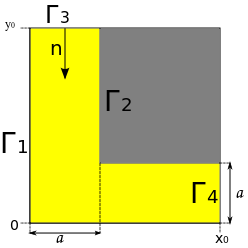
We have a linear equation in ch.p. We will solve it without flow, i.e. at the boundaries 1, 2, 4, the derivative is normal to the wall 0, and at the border 3, the concentration is determined by a given function g (t). Thus we get a mixed boundary value problem. We will solve it by the method of finite differences (very inefficient, but simple).

About parallelization

To solve this problem, I used openMPI / intelMPI (a separate post should be devoted to comparing compilers in practice). I will not go deeper into the numerical scheme, because there is Wikipedia and I will only say that I used an explicit scheme. I used the block distribution of the area so that each stream is given several areas and if the data that is transmitted from the previous area is zero, then the area is not considered. Extreme columns / rows of blocks are designed to receive data from neighboring streams.

Grid parameters used in calculations

Number of nodes in the grid: 3 * 10 ^ 6
Grid step: 0.0007.
Physical diffusion time: 1 s
Time step: 6.5 * 10 ^ -7
D: 0.8
The initial concentration at the boundary is 3 0.01 mol.

A little about the law Amdala

Jim Amdal formulated a law illustrating the performance limitations of a computing system with an increase in the number of calculators. Suppose you need to solve any computational problem. Let α be the fraction of the algorithm that runs sequentially. Then, respectively, 1-α is executed in parallel and can be parallelized on p-nodes, then the acceleration obtained on the computing system can be obtained as

Let's turn to the most interesting to the results and results of parallelization.

Runtimes on a different number of threads

number percent	one	2	eight	sixteen	32	64	128
time min	840	480	216	112	61	46	41

We approximate the calculation times by the Amdal law.

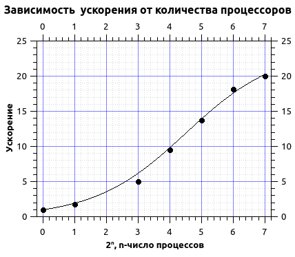
From the approximation, I got the sequential code rate of about 4.2% and the maximum acceleration about 20 times. As can be seen from the graph, the curve goes to the plateau, from this we can conclude that the maximum acceleration is reached and further dragging the number of processors is impractical. Moreover, in this case, with an increase in the number of processes over 200, I received a decrease in acceleration, this is due to the fact that with an increase in the number of processes, their irrational use begins, i.e. the number of rows in the grid becomes commensurate with the number of processes and more time is spent on exchanges, and this time makes a significant contribution during the calculations.

Some notes

In the UK, the sbatch task management system is used and there are several test queues test, regular4, regular6, gputest, gpu. For this task, I used the regular4 queue in which the waiting time can reach three days (in practice, the waiting time is 17-20 hours).