What happens in the brains of the neural network and how to help them

Recently, on Habré has appeared many articles on neural networks. Of these, articles about the Rosenblatt Perceptron seemed very interesting: Rosenblatt's Perceptron - what is forgotten and invented by history? and What is the role of the first "random" layer in the Rosenblatt perceptron . In them, as in many others, a lot has been written about how networks cope with problem solving, and generalize to some extent their knowledge. But I would like to somehow visualize these generalizations and the decision process. To see in practice what the perceptron learned there, and to feel how successfully he succeeded. It is possible to experience bitter irony regarding the achievement of mankind in the field of AI.
The language we will have is C #, just because I recently decided to learn it. I analyzed two of the most simple examples: the Rosenblatt single-layer perceptron, trained by error correction, and Rumelhart's multilayer perceptron, trained by the method of back propagation of error. For those who, like me, it became interesting what they actually learned there, and how well they are really able to generalize - welcome under the cat.

CAUTION! A lot of pictures. Pieces of code.

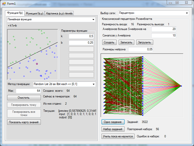
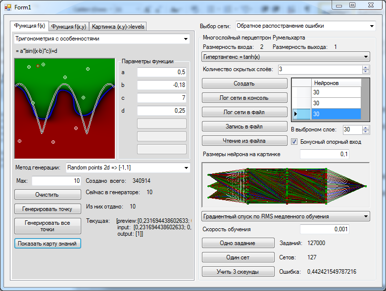
First I want to invite you to admire the process of learning a neural network. Every frame after 1000 learning points. Indicates the speed of learning and the root mean square error for this thousand cycles.

From the code I will show only what may be useful to others who want to do everything with their own hands or check the correctness of my conclusions. The code of important elements is torn from the root of the test project in which it was launched, so there may be links to elements that I don’t cite. But the code is working, all the pictures are screenshots from my training project.
')
First you need to choose a task, such that it looked at it, and it immediately became clear whether the perceptron had learned anything and anything. Take two coordinates (x and y), and assign many random points to them. This will be the input data. Let's draw some graph and ask the perceptron to determine if the point is above or below this graph. But Rosenblatt’s perceptron works in integers, and indeed the problem is too simple. Then let's round each coordinate to an integer and present it in binary form: one digit-one entry. For consistency, all the examples consider the range of coordinates (0.1), so that before rounding it should be multiplied by the maximum integer value.

For example, imagine each coordinate is a two-bit number. A pair of random numbers (0.2, 0.7) pointing to a point above the graph, then after rounding it will go to (1.3) and give us the following example:

new double[]{0.2, 0.7} => new NeuralTask { Preview = new double[]{0.25, 0,75, 1}, Input=new double[] {0,1,1,1}, Output=new double[]{1}}

The function that converts random numbers into training examples looks like this:

Conversion function

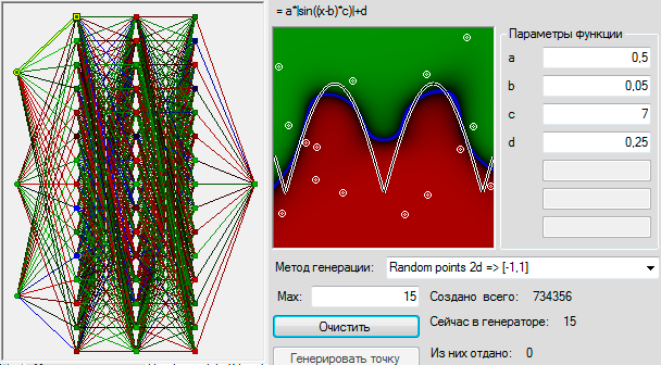
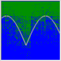
  var Convertion = (double[] random, double value) => { var input = new double[]{Math.Floor(random [0]*0x4)/0x4, Math.Floor(random [1]*0x4)/0x4}, byte x = (byte)(input[0] * 4); byte y = (byte)(input[1] * 4); int res = (y > value * 4 ? 1 : 0); return new NeuralTask() { input = new double[4]{ (x&2)>>1, x&1, (y&2)>>1, y&1}, output = new double[1] { res }, preview = new double[3] { input[0], input[1], res } }; };

Here it is necessary to clarify that all this was done for educational and research purposes, therefore it was not optimized for speed and unearthly beauty, but somewhere it was written so that it was convenient to program any conceivable perceptron. Therefore, in particular, the input and output data are in double. It turns out such a simple picture. Well, or a little more complicated, if each axis is chopped into 256 sections, and the function is more complicated:

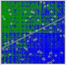
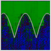
Hereinafter, the green color - values are greater than zero, the more saturated, the greater the number, red - values less than zero, blue - values equal to 0 and their closest surroundings.

Source

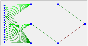
Our perceptron itself consists of a synapse:

class Synaps

  public class Synaps { private double weight; /// <summary>   </summary> virtual public double Weight { get { return weight; } set { if (weight != value) { weight = value; if (axon != null) ChangeActionPotentialHandler(axon.ActionPotential); } } } /// <summary>    . ,  ,   ,     ,      .</summary> private IAxon axon; //   ,    . public IAxon Axon { get { return axon; } set { //    ,       . if (axon != null) axon.RemoveChangeActionPotentialHandler(ChangeActionPotentialHandler); axon = value; if (axon != null) { axon.AddChangeActionPotentialHandler(ChangeActionPotentialHandler); ChangeActionPotentialHandler(axon.ActionPotential); } } } public double ActionPotential; /// <summary>  ,     .</summary> protected Action WhenActionPotentialhanged; public void AddActionPotentialChangeHandler(Action handler) { WhenActionPotentialhanged += handler; } public void RemoveActionPotentialChangeHandler(Action handler) { WhenActionPotentialhanged -= handler; } virtual protected void ChangeActionPotentialHandler(double axonActionPotential) { ActionPotential = axonActionPotential * weight; //      ,       . if (WhenActionPotentialhanged != null) WhenActionPotentialhanged); //          } }

Nothing unexpected, except that the numbers are stored in double and instead of the standard event used custom. Now the neuron. Neurons here all together correspond to the IAxon interface:

interface IAxon

  public interface IAxon { /// <summary>  .</summary> double ActionPotential { get; } /// <summary>    .</summary> void AddChangeActionPotentialHandler(Action<double> handler); void RemoveChangeActionPotentialHandler(Action<double> handler); /// <summary>,        .</summary> PointF Position { get; set; } /// <summary>      .</summary> string Name { get; set; } }

Nothing too unexpected, except for Position, showing where the neuron is to draw.

The input uses sensory neurons, which can be set directly:

class SensoryNeuron

  public class SensoryNeuron : IAxon { protected double actionPotential; public double ActionPotential { get { return actionPotential; } set { if (actionPotential != value) { actionPotential = value; if (WhenChangeActionPotential != null) WhenChangeActionPotential(actionPotential); } } } }

Finally, the neuron itself is in a rather generalized form:

class Neuron

  /// <summary> .     </summary> public class Neuron : IAxon { /// <summary>  ,      .    ,     ,     .</summary> public Synaps[] Synapses = new Synaps[0]; /// <summary>  , ,            .</summary> protected bool synapsPotentialChanged = false; /// <summary>      .  ,  ,   . </summary> public void AppendSinaps(Synaps target) { //     .  , , ,      ,     . Synapses = Synapses.Concat(new Synaps[1] { target }).ToArray(); target.AddActionPotentialChangeHandler(ChangeSynapsPotentialHandler); //   . synapsPotentialChanged = true; } virtual protected void ChangeSynapsPotentialHandler() { synapsPotentialChanged = true; } /// <summary>   .     ,    .</summary> protected DTransferFunction transferFunctionDelegate; public virtual DTransferFunction TransferFunction { get { return transferFunctionDelegate; } set { transferFunctionDelegate = value; } } /// <summary>             . </summary> public virtual void Excitation() { if (!synapsPotentialChanged) return; //        synapsPotentialChanged = false; synapsPotentials = 0; for (int i = 0; i < Synapses.Length; i++) synapsPotentials += Synapses[i].ActionPotential; double newValue = transferFunctionDelegate(synapsPotentials); if (actionPotential != newValue) { //        . ,   . actionPotential = newValue; if (WhenChangeActionPotential != null) WhenChangeActionPotential(actionPotential); } } }

Here:

Activation function

  /// <summary>        . </summary> /// <param name="argument">  </param> /// <returns>    </returns> public delegate double DTransferFunction(double argument); DTransferFunction BarrierTransferFunction = (double x) => x <= 0 ? 0 : 1;

Finally, from all of this, the neural network and its learning algorithm are obtained:

class NeuralNetwork, PerceptronClassic, ErrorCorrection

  abstract public class NeuralNetwork { /// <summary>  </summary> public SensoryNeuron[] Input = new SensoryNeuron[0]; /// <summary> ///            ,    .      . ///           ,          . /// </summary> public Neuron[] ExcitationOrder = new Neuron[0]; /// <summary>  </summary> public Neuron[] Output = new Neuron[0]; /// <summary> ,       </summary> /// <param name="input">   - </param> /// <param name="output">   </param> abstract public void create(uint input, uint output); public void execute(double[] data) { //               for (int i = 0; i < Input.Length && i < data.Length; i++) { Input[i].ActionPotential = data[i]; } for (int i = 0; i < ExcitationOrder.Length; i++) ExcitationOrder[i].Excitation(); } public double[] Result() { // return output.Select(s => s.ActionPotential).ToArray(); //TODO     Linq  . double[] res = new double[Output.Length]; for (int i = 0; i < res.Length; i++) res[i] = Output[i].ActionPotential; return res; } } public class PerceptronClassic : NeuralNetwork { //     ,    public int neuronCountsOverSensoric = 15; //     public int ANeuronSynapsCount; //      public Neuron[] Layer; //        override public void create(uint inputCount, uint outputCount) { rnd = rndSeed >= 0 ? new Random(rndSeed) : new Random(); //   this.Input = new SensoryNeuron[inputCount]; for (int i = 0; i < inputCount; i++) Input[i] = new SensoryNeuron() {Name = "S" + i}; //    -  Layer = new Neuron[inputCount + neuronCountsOverSensoric]; for (int i = 0; i < Layer.Length; i++) { //    Layer[i] = new RosenblattNeuron(); //         SensoryNeuron[] sub = Input.OrderBy((cell) => rnd.NextDouble()).Take(ANeuronSynapsCount).ToArray(); //   ,    for (int j = 0; j < sub.Length; j++) { Synaps s = new Synaps(); s.Axon = sub[j]; s.Weight = rnd.Next(2) * 2 - 1; Layer[i].AppendSinaps(s); } } //     . for (int i = 0; i < Layer.Length; i++) Layer[i].Name = "A" + i; //   -   Output = new Neuron[outputCount]; for (int i = 0; i < Output.Length; i++) { Output[i] = new RosenblattNeuron(); Output[i].Name = "R" + i; //        for (int j = 0; j < Layer.Length; j++) { Synaps s = new Synaps(); s.Axon = Layer[j]; Output[i].AppendSinaps(s); //   0 } } //       int lastIndex = 0; ExcitationOrder = new Neuron[Layer.Length + Output.Length]; foreach (Neuron cell in Layer) ExcitationOrder[lastIndex++] = cell; foreach (Neuron cell in Output) ExcitationOrder[lastIndex++] = cell; } } /// <summary>   .</summary> public class ErrorCorrection : LearningAlgorythm { // ,        override protected double LearnNet(double[] required) { double error = 0; for (int i = 0; i < required.Length && i < net.Output.Length; i++) { if (required[i] != net.Output[i].ActionPotential) { error += 1; //     for (int j = 0; j < (net as PerceptronClassic).Layer.Length; j++) //    ,   if ((net as PerceptronClassic).Layer[j].ActionPotential > 0) //      foreach (RosenblattNeuron cell in net.Output) //    ,       //    – ,   ,   – .    . cell.Synapses[j].Weight += required[i] <= 0 ? -1 : 1; } } return error; } /// <summary>       </summary> public void LearnTasksSet() { if (data == null) { Console.WriteLine("  "); return; } data.Reset(); LearnedTaskSetsCount++; ErrorsInSet = LearnedTasksInSetCount = 0; int max = 1000; while (data.MoveNext() && --max >= 0) LearnCurrentTask(); //     ,    . } /// <summary>         .</summary> /// <param name="loops">    </param> public void LearnSetManyTimesUntilSuccess(int loops) { for (int i = 0; i < loops; i++) { LearnTasksSet(); if (ErrorsInSet == 0) { break; } } } }

The data source is Enumerable<NeuralTask> and with each Enumerable<NeuralTask> it rearranges points in a sequence in random order.

Everything is ready, you can run.

For the simplest problem, two bits per axis, so that we were lucky to find a suitable separable decomposition, we had to add 8 more neurons to layer A than 12 inputs. A suitable decomposition was found on the third attempt. Perceptron correctly classified all 16 possible values.

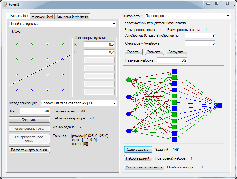
Here you can see that there are only 16 possible values, and I generated more. So that random numbers are guaranteed to cover all possible options.

Since everything is so wonderful, let's move on to a slightly more complicated task, where we have 256 options for each axis. Function consider the simplest. Let's generate, for a start, 64 points. In the layer of neurons only 20 more than the inputs - 36 pieces. And immediately success.

And now we will do the most interesting. We take the network we received and draw in the picture all the possible values that the network gives at all points. And here it turns out the saddest thing. The level of generalization achieved by the network is not very impressive.

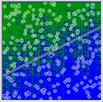
It turns out that the network in a very general way represents what pattern lies behind the points given to it. Let's try to provide the network with more complete data about the function being studied. Generate 256 points. 36 neurons, as last time, are not enough for the network to encounter a suitable linearly separable decomposition. Now we needed to create 70 associative neurons, drive out the training set of tasks 615 times and vacuum the cooler so that the processor does not overheat for joy in just one second of training. The generalization achieved by the network has become better, but it can be seen with the naked eye that the improvement obtained is disproportionately expended.

In the hearts, we cover the space with 2048 points. By force we create already 266 neurons in the associative layer, select the optimal number of synapses per neuron (it turns out 8) learn the set 411 times (until the network stops to make mistakes) and look at the achieved result.

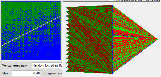
I don’t know about you, but I don’t see any quality improvement. The network regularly memorizes all values by heart, in no way approaching the generalization of the pattern proposed to it. And in general it is clear that the nature of the profound conclusions made by the network is not so much dependent on the nature of the task before it.

Thanks, of course, that I managed to at least learn it. It seems that the theorems are correct, and if I have a sufficient number of neurons, I can force the network to memorize at least all 65536 variants possible for this task, but we will need approximately 1500-2000 neurons and water cooling for this. In order to remember all the information contained in such a network, we need 5 bits for each synapse (4 bits for the axon number and weight bits), 16 bits for each neuron for the axon weight and 40 bits for all synapses. And one teaching example weighs 17 bits. In our example with 2048 points, it turns out that the training information weighs only two times more than the information about the received network.

Convenient tasks

So what's the problem? What is the reason for such a sad picture? Let's try to solve the problem analytically. Suppose we have a perceptron, but only the weights of the first layer, as well as the second, are amenable to learning. In the second layer, we have only three neurons. The first is connected to the first 8 inputs and has not a barrier, but simply a linear activation function. The second neuron is the same, but is only responsible for converting the second 8 bits to normal coordinates. The third is connected with all, has a barrier function and is intended to give 1 if at least one input has at least something. In the next layer, two of the neurons are summed, again without a barrier function, but with very important weighting factors reflecting the parameters of the function. And finally, the last neuron will compare two input signals. Simple, logical and not a bit interesting. However, this is almost the minimum possible number of neurons and synapses involved for a given task. And now try to imagine how many neurons you need to express any of these operations in a single-layer perceptron, whose synapse weights in the first layer can only be -1 and 1. For example, casting 8 bits to one number. I'll tell you - you need about 512 pieces of neurons, and we haven't started comparing this yet.

That is, the problem is not that Rosenblatt's perceptron cannot learn this data set. The problem is that doing it is very, very uncomfortable. Anyone who is friends with the theorem of large numbers can try to estimate what the probability is to find a linearly separable decomposition suitable for this. Rosenblatt's Perceptron is convenient to solve problems that are well represented in the form of a spotted blue-green diffuse gradient, but everything becomes sad when it is not.

And what about Rumelhart's multilayer perceptron?

But what if only Rosenblatt’s single-layer perceptron has problems, and a multi-syllable perceptron that is trained using the error propagation method will be very good, and even magical? Let's try.

Source

First, now we will add a function to calculate the first derivative of the neuron activation function at current values. All of this can be scary to optimize and syncline the calculation of the derivative directly into the formula in which it will be applied, but our task is not to speed things up, but to figure out how it works. Therefore, a separate function:

Derivative of the activation function

  /// <summary>      . </summary> /// <param name="argument">  </param> /// <param name="funcResult">  ,    </param> /// <returns>       .</returns> public delegate double DTransferFunctionDerivative(double argument, double funcResult);

As a sigmoid, we use, for example, Hypertangent:

 DTransferFunction Function = (x) => Math.Tanh(x), DTransferFunctionDerivative Derivative = (x, th) => (1 - th) * (1 + th)

Now the neuron itself. It differs only in that for each calculation the value also calculates the derivative of it from the sum of the input signals, and the presence of a variable in which the value used for back propagation of the error will be stored.

class NeuronWithDerivative

  public class NeuronWithDerivative : Neuron { /// <summary>    .           .</summary> protected DTransferFunctionDerivative transferFunctionDerivativeDelegate; /// <summary></summary> override public DTransferFunctionDerivative TransferFunction { get { return transferFunctionDerivativeDelegate; } set { transferFunctionDerivativeDelegate = value; } } /// <summary>        </summary> protected double actionPotentialDerivative = 0; /// <summary>        .</summary> public double ActionPotentialDerivative { get { return actionPotentialDerivative; } } /// <summary>     . ,    .   .</summary> public double BackProprigationParametr = 0; public override void Excitation() { base.Excitation(); actionPotentialDerivative = transferFunctionDerivativeDelegate(synapsPotentials, actionPotential); } }

I, lately, like to use LINQ, because it's easier and faster to write experimental code. For the convenience of this business, my little home function expands its capabilities. I use it instead of List.ForEach so that the call is beautiful and single-line.

static class Tools

  static class Tools { /// <summary>         .</summary> /// <param name="source">   .</param> /// <param name="func">,   .</param> public static void Each<SequenceType>(this IEnumerator<SequenceType> source, Action<SequenceType> func) { while (source.MoveNext()) func(source.Current); } /// <summary>             .</summary> /// <param name="source">   .</param> /// <param name="func">,   .     -   .      .   -  .</param> public static void Each<SequenceType>(this IEnumerator<SequenceType> source, Action<SequenceType, int> func) { for (int i = 0; source.MoveNext(); i++) func(source.Current, i); } /// <summary>         .</summary> /// <param name="source">   .</param> /// <param name="func">,   .</param> public static void Each<SequenceType>(this IEnumerable<SequenceType> source, Action<SequenceType> func) { source.GetEnumerator().Each(func); } /// <summary>             .</summary> /// <param name="source">   .</param> /// <param name="func">,   .     -   .      .   -  .</param> public static void Each<SequenceType>(this IEnumerable<SequenceType> source, Action<SequenceType, int> func) { source.GetEnumerator().Each(func); } }

class RumelhartPerceptron

  //          . public class RumelhartPerceptron : NeuralNetwork { /// <summary>   .  .</summary> DTransferFunctionDerivative TransferFunctionDerivative; /// <summary>    ,      </summary> public int[] NeuronsCount = new int[0]; override public void create(uint input, uint output) { //  . Input = (new SensoryNeuron[input]).Select((empty, index) => new SensoryNeuron(){Name = "S[" + index + "]"}).ToArray(); //     Func<string, NeuronWithDerivative> create = (name) => { NeuronWithDerivative neuron = new NeuronWithDerivative(); neuron.Name = name; neuron.TransferFunction = TransferFunction; neuron.TransferFunctionDerivative = TransferFunctionDerivative; return neuron; }; Func<IAxon, Synaps> createSynaps = (axon) => { Synaps s = new Synaps(); s.Axon = axon; return s; }; /// <summary>  </summary> //       NeuronWithDerivative[][] Layers = NeuronsCount.Select((count, layer) => Enumerable.Range(0, count).Select(index => create("A[" + layer + "][" + index + "]")).ToArray()).ToArray(); //      //   Output = Enumerable.Range(0, (int)output).Select(index => create("R[" + index + "]")).ToArray(); //         . Layers[0].Each(neuron => { Input.Select(createSynaps).Each(synaps => { neuron.AppendSinaps(synaps); }); }); //  ,    ,      . Layers.Skip(1).Each((layer, layerIndex) => { layer.Each(neuron => { Layers[layerIndex].Select(createSynaps).Each(synaps => { neuron.AppendSinaps(synaps); }); }); }); //        Output.Each(neuron => { Layers.Last().Select(createSynaps).Each(synaps => { neuron.AppendSinaps(synaps); }); }); //      ExcitationOrder = Layers.SelectMany(layer => layer).Concat(Output).ToArray(); //       -1  +1 Random rnd = new Random(); ExcitationOrder.Each(neuron => neuron.Synapses.Each(synaps => synaps.Weight = rnd.NextDouble() * 2 - 1)); } }

, , . LINQ , . , , .

class BackPropagationLearning

  public class BackPropagationLearning : LearningAlgorythm { // ,     public double LearningSpeed = 0.01; override protected double LearnNet(double[] required) { double[] errors = net.Output.Select((neuron, index) => neuron.ActionPotential - required[index]).ToArray(); //     .     ,                . net.ExcitationOrder.Cast<NeuronWithDerivative>().Each(neuron => { neuron.BackProprigationParametr = 0; }); //   BackProprigationParametr    dE/dS[i] = dE/dO[i] * F'[i](S[i]) //          . BP[i] = dE/dO[i] * F'[i] = 2*(O[i]-T[i])*F'[i]; net.Output.Cast<NeuronWithDerivative>().Each((neuron, index) => { neuron.BackProprigationParametr = 2 * errors[index] * neuron.ActionPotentialDerivative; }); //      ,       BP[j] = SUM( dE/dO[i] * F'[i] * W[j,i] ) * F'[j] = SUM ( BP[i] * W[j,i] * F'[j]) net.ExcitationOrder.Reverse().Cast<NeuronWithDerivative>().Each(neuron => { neuron.Synapses.SkipWhile(synaps => !(synaps.Axon is NeuronWithDerivative)).Each(synaps => { (synaps.Axon as NeuronWithDerivative).BackProprigationParametr += neuron.BackProprigationParametr * (synaps.Axon as NeuronWithDerivative).ActionPotentialDerivative * synaps.Weight; }); }); //     ,    delta W[i,j] = -speed * dE/dS[j] * X[i]; net.ExcitationOrder.Reverse().Cast<NeuronWithDerivative>().Each(neuron => { neuron.Synapses.Each(synaps => { synaps.Weight += -LearningSpeed * neuron.BackProprigationParametr * synaps.Axon.ActionPotential; }); }); //     . (        ,  ). return errors.Select(e => e * e).Average(); } public void LearnSomeTime(int sek) { DateTime begin = DateTime.Now; while (TimeSpan.FromTicks(DateTime.Now.Ticks - begin.Ticks).Seconds < sek) { LearnTasksSet(); } } }

Here is the code. It differs from the canonical implementation only in that the learning rate is not sewn into the back propagated error, but multiplied by the change in weight immediately before use. We minimize the sum of the squares of errors, as Wikipedia teaches us, which in this part was filled with habrovchanami.

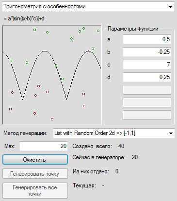
What is the task of letting our network begin? Let's take the same x and y from the [0,1] section, at the points that are higher than the graph, we will expect the network output to be +1, at the points below the -1 graph. In addition, we will make more than one fixed sequence of training examples, and we will create a new training example each time anew, so that it cannot be said that the network did not have information about some important area of space. We give the created packs of variables of 1000 pieces per set. In the preview, not one point is shown, but several last ones created only for beauty. It turns out somehow.

Create a neural network. Wikipedia tells us that three layers should be enough. In order not to seem small, let's fix 30 neurons each in a layer. Let's try to teach with some similarity of the annealing simulation algorithm, gradually manually reducing the speed of learning, as the root-mean-square error in the last 1000 training examples ceases to improve. Programming annealing was too lazy, because my article is not about that. We train, we train, and finally, when the quality of the network ceases to improve, we draw in the picture the values that the network will produce for each of our points in the 1x1 square.

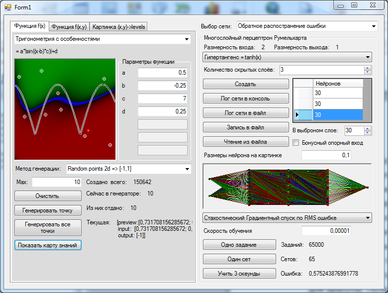
Well, as for me, this is a rather modest result, and this is also the best of 5 attempts, he at least has two concavities, this is not always possible for networks of this size. Pay attention to the picture with the results of 4 more attempts in a row.

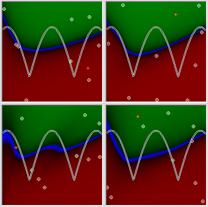
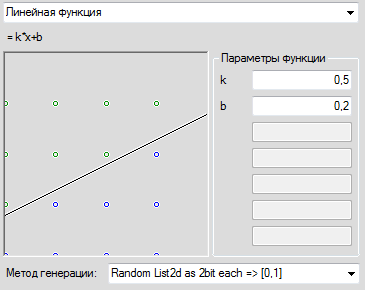
All attempts give, in principle, a similar result, and at all the picture is filled up to the left, despite the fact that the desired graph in all these cases is located symmetrically. The dullness of the network can be attributed to many different reasons, including errors in the programmer’s DNA, but the fact that it’s convenient to roll up the networks to the left should have some kind of rational explanation. So maybe we made a mistake somewhere? Let's offer the network to cope with quite a banal task - we give a simple linear relationship as a problem. We look.

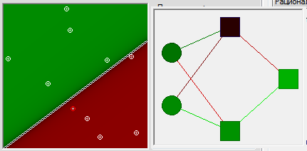
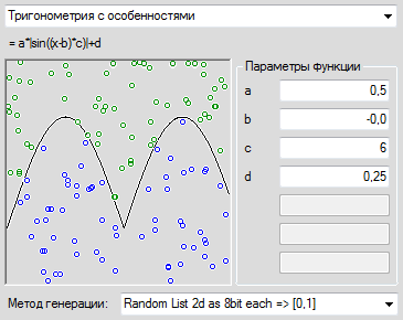
All is well, all is right. By manually tracking the state of the variables, you can verify that the algorithm is working correctly. Then we give the puzzle a little more difficult. The result can be seen in the following picture.

Full fiasco

We look at it and understand that something is wrong here. The task is not that simple, it is primitive. But the network is decisively unable to find its solution in any approximation.

Have you guessed why? It clearly follows from the picture why this is impossible, and at the same time the answer to the question why all the decisions from the previous picture were left to the left.

If we try to design a solution to this problem analytically - manually, with a pen and paper, we will very quickly encounter the correct answer. If you have a neuron with a symmetric sigmoid, you will not force it to do the transformation output = k * input + b with any tricks. A neural network with a symmetric with respect to zero sigmoid at the point (0,0) cannot output anything except 0 (hello, by the way, Rosenblatt's perceptron convergence theorem, there is also such a special point there).

To solve this problem, we can add another input to the neural network, and give it a constant value of 1, independent of the input data. And then the network, as if by magic, is getting smarter and is learning the task before it in the shortest possible time and with incredible accuracy.

And here the most interesting begins.

But can there be a good approximation without an additional reference input? Will we be able to come up with a solution for the network topology from the previous picture? It turns out that this is possible.

Brain against back distribution

In the course of the network, I suggested several times to find a solution for the network manually. Now we will analyze one of these solutions in detail.

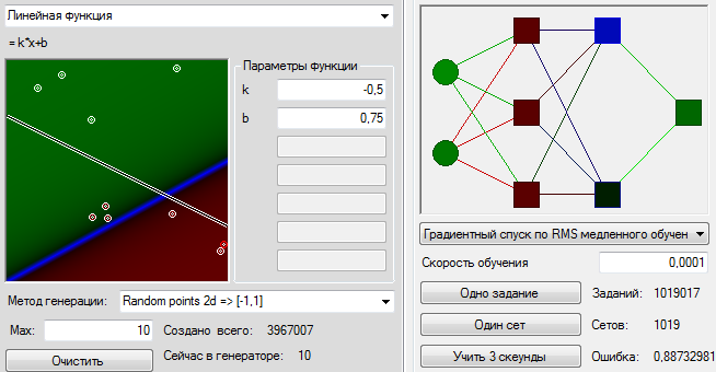
Our network inputs are called S [0] and S [1], the neurons of the first layer are A [0] [1], A [0] [2] and A [0] [3], respectively, the next layer is A [1] [ 0] and A [1] [1] and, finally, the output of R [0]. What did we lack the last time we tried to solve the problem analytically? We lacked a reference constant. Take one neuron, for example, A [0] [0] and hang very high weights at synapses, for example, 1000 each. In addition to a small area in the immediate vicinity of 0, the action potential on this neuron will be equal to 1.

What's next?A [0] [1], we will transmit information about the first coordinate and have weights of synapses respectively 1 and 0, neuron A [0] [2] - information about the second coordinate, and have synapses with weights 0 and 1. We want so that the function of the first coordinate is compared with the second coordinate. To do this, we simply transmit the second coordinate to the second neuron of the second layer. Assign synapse weights, respectively, 0.0 and 1. And in the first synapse of the second layer, we want to get the value of k * xb. Accordingly, k = -0.5 b would be equal to 0.75 if the activation functions of the neurons did not bend the values. About the input x = 1 on the neuron A [0] [1] there will be only 0.76 potential. So for comparison, we need about b = 0.65. With this value, the neuron A [1] [0] should have approximately the same value as the neuron A [1] [1] for points lying on our original line. Well now,in order to compare these two values, let's endow the output neuron R [0] with values at -1 and 1. Synapses. Let's display what we have in the picture. Right beauty! Blue zero values are approximately where they are needed. Top green. Red below. Of course, for the time being it is not green enough and not red enough. However, the final fine-tuning of the weights of synapses will be able to do the error back-propagation algorithm not only worse, but better than me. We start the algorithm, and after a small number of steps, we have a fairly tolerable approximation.However, the final fine-tuning of the weights of synapses will be able to do the error back-propagation algorithm not only worse, but better than me. We start the algorithm, and after a small number of steps, we have a fairly tolerable approximation.However, the final fine-tuning of the weights of synapses will be able to do the error back-propagation algorithm not only worse, but better than me. We start the algorithm, and after a small number of steps, we have a fairly tolerable approximation.

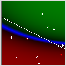
Here you can see how the network looks like:

XML to which the finished network is exported

 <rumelhart> <input> <SensoryNeuron name="S[0]" potential="0,0396039603960396"/> <SensoryNeuron name="S[1]" potential="0,232673267326733"/> </input> <excitationOrder> <Neuron name="A[0][0]" potential="1"> <synaps weight="999,800400355468" axon="S[0]" potential="39,5960554596225" /> <synaps weight="999,545226476388" axon="S[1]" potential="232,5674536851" /> </Neuron> <Neuron name="A[0][1]" potential="0,116342019068401"> <synaps weight="1,13712492177543" axon="S[0]" potential="0,0450346503673436" /> <synaps weight="0,308744483692756" axon="S[1]" potential="0,0718365877898986" /> </Neuron> <Neuron name="A[0][2]" potential="0,29693700450834"> <synaps weight="-0,0240967983057654" axon="S[0]" potential="-0,000954328645772886" /> <synaps weight="1,31992553337836" axon="S[1]" potential="0,307111386479124" /> </Neuron> <Neuron name="A[1][0]" potential="0,683083451961352"> <synaps weight="1,02404884109051" axon="A[0][0]" potential="1,02404884109051" /> <synaps weight="-0,649771926175146" axon="A[0][1]" potential="-0,0755957778251805" /> <synaps weight="-0,382508459201211" axon="A[0][2]" potential="-0,113580916074308" /> </Neuron> <Neuron name="A[1][1]" potential="0,0324886810522597"> <synaps weight="-0,404744328902586" axon="A[0][0]" potential="-0,404744328902586" /> <synaps weight="0,161865952018599" axon="A[0][1]" potential="0,0188318116762727" /> <synaps weight="1,40909563283595" axon="A[0][2]" potential="0,418412636280091" /> </Neuron> </excitationOrder> <output> <Neuron name="R[0]" potential="-0,707598983150799"> <synaps weight="-1,36308077548559" axon="A[1][0]" potential="-0,931097921420856" /> <synaps weight="1,50019153981243" axon="A[1][1]" potential="0,0487392444542643" /> </Neuron> </output> </rumelhart>

There is one interesting point in all this manual solution. The fact is that the perceptron, driven by the error back-propagation algorithm, in principle could not find this solution in our situation. Because between the initial state, when all synapses have an initial value in the range [-1,1] and a final one, at which two synapses weigh a lot, there is a very wide gap filled with very bad solutions, and the gradient descent algorithm will carefully push the network out this abyss. As I call this solutions have high incoherence. The annealing simulation algorithm may accidentally throw the network into that area, but for this, the annealing temperature must be high (for the chance to throw the network so far) and very quickly decrease so that it does not immediately drop out. And since the weights of a part of synapses should be large, while others, on the contrary, have very little difference, we should accidentally hit not only large values, but also quite by chance, it’s good to get into small values, and the algorithm should freeze very sharply when that - I found this because the area of suitable solutions is very narrow. Even at a learning rate of 0.0001, a simple stochastic gradient descent can easily throw a network out of it. In general, there is a solution, but I just cannot find its network.

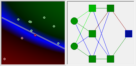
Although, as you probably noticed, if you give a network three layers of 30 neurons, the network can independently find a way to partially solve the zero point problem. Although doing it is very uncomfortable. If we give the network an additional reference input, the picture is no longer skewed to one side. But even more, the very process of finding a solution becomes much more productive - free from the need to spend half of its priceless neurons to create a constant, the network was able to fully turn around and act as if it were on one layer and a few dozen more neurons. Details can be admired in the picture.

And the solution to this problem is not the only way to improve the quality of network training at times by manipulating the topology. I showed it precisely because it could be beautifully demonstrated with an analytical solution using a simple example.

Interestingly, adding one input with a constant significantly improves network performance even in cases where neighborhoods of zero value do not fall into the input task with which we train the network. For example, below I proposed a regular network, and a network with an additional input the same task and the same varying learning speed. Moreover, the entire graph was shifted by one axis on both axes, so that the input of the network received values in the range from 1 to 2. The results speak for themselves.

Finally, if we feed this algorithm the first initial integer problem proposed by the Rosenblatt perceptron, the results will be noticeably better than last time. But we must also take into account the fact that in a multilayer perceptron there are 30 more neurons of synapses, because writing data on the network requires significantly more bytes than the original data itself weigh.

findings

The Rosenblatt perceptron can be taught only by such knowledge, which at the point with zero inputs implies zero output. If you were interested in the convergence theorem, but did not notice that this follows from it, then reread it more carefully. I would never believe that Rosenblatt or Minsky could err in the evidence;
, . , , ;
, . , , , ;
, , . , ;
The fact that a task can be solved in principle using a neural network does not mean at all that this solution can be achieved from the initial state of the network. Moreover, the connectedness of the solution space should be considered as one of the main factors in the training of neural networks;
Adding to the input a simple constant value in very many cases greatly improve the quality of the network for a variety of tasks.

UPD: Fixed a bug in the code. It would seem critical, in the implementation of reverse distribution, but for some reason all the results of the network did not change. It surprises me even more.

Source: https://habr.com/ru/post/219647/

All Articles