Harmonic vibrations
On Habré there were several articles on the Fourier transform and about all sorts of beautiful Digital Signal Processing (DSP) types, but an inexperienced user is completely unclear why all this is needed and where, and most importantly, how to apply it.
Frequency response noise.
Personally, after reading these articles (for example, this one ) I didn’t understand what it was and why it was needed in real life, although it was interesting and beautiful.
It would be desirable not just to look at beautiful pictures, but to say so, to feel in your gut, what and how it works. And I will give a concrete example with the generation and processing of sound files. It will be possible to listen to the sound and look at its spectrum, and understand why this is so.
The article will not be of interest to those who own the theory of functions of a complex variable, DSP, and other terrible topics. It is more likely for the curious, schoolchildren, students and their sympathizers :).
')
Immediately make a reservation, I am not a mathematician, and I can even say many things incorrectly (correct with a personal message), and I am writing this article based on my own experience and my own understanding of current processes. If you are ready, then go.
If we recall a school course in mathematics, then we used a circle to build a sine graph. In general, it turns out that the rotational motion can be turned into a sinusoid (like any harmonic oscillation). The best illustration of this process is given in wikipedia.
Harmonic vibrations
Those. in fact, the sine plot is obtained from the rotation of the vector, which is described by the formula:
where A is the vector length (amplitude of oscillations), φ is the initial angle (phase) of the vector at time zero, ω is the angular velocity of rotation, which is equal to:
ω = 2 πf, where f is the frequency in Hertz.
As we can see, knowing the signal frequency, amplitude and angle, we can build a harmonic signal.
Magic begins when it turns out that the representation of absolutely any signal can be represented as a sum (often infinite) of various sinusoids. In other words, in the form of a Fourier series.
I will give an example from the English Wikipedia . For example, take a ramp.
Ramp
Its sum will be represented by the following formula:
If we successively sum up, take n = 1 first, then n = 2, etc., we will see how our harmonic sinusoidal signal gradually turns into a saw:
Probably the most beautiful thing is illustrated by one program I found in the open spaces of the network. It was already mentioned above that the sine graph is a projection of a rotating vector, but what about more complex signals? This, oddly enough, the projection of a set of rotating vectors, or rather their sum, and it looks like this:
Vectors draw a saw.
In general, I recommend to go by the link and try to play with the parameters, and see how the signal changes. IMHO more visual toys for understanding, I have not yet met.
It should also be noted that there is an inverse procedure that allows to obtain from this signal the frequency, amplitude and initial phase (angle), which is called the Fourier Transform.
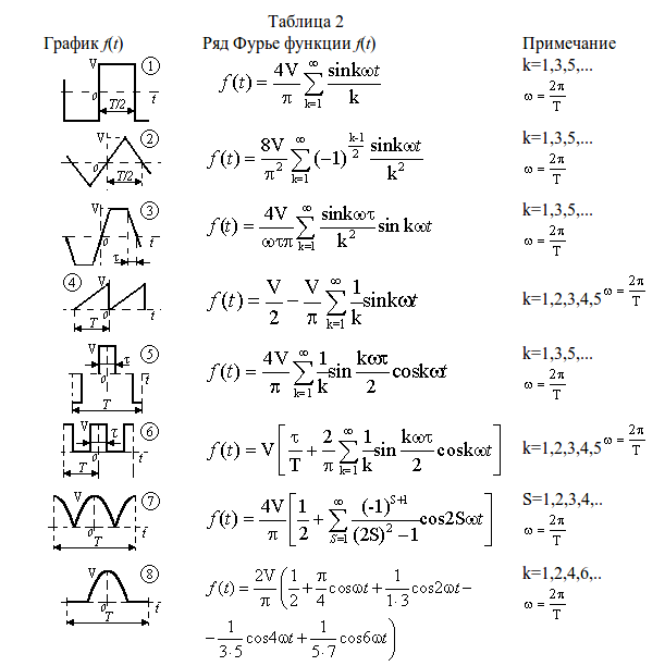
Fourier series decomposition of some known periodic functions ( from here )
I will not dwell on it in detail, but I will show how this can be applied in life. In the list of references I will recommend something where you can read more about the materiel.
It seems to me that each student wonders, sitting at a lecture, for example, on matan: why do I need all this nonsense? And as a rule, not finding an answer in the foreseeable future, unfortunately, loses interest in the subject. Therefore, I will immediately show the practical application of this knowledge, and you will already master this knowledge yourself :).
All further I will implement on it. I did everything, of course, under Linux, but I didn’t use any specifics; in theory, the program will compile and work under other platforms.
To begin with we will write the program for formation of the sound file. Wav file was taken as the easiest. Read about its structure here .
In short, the structure of the wav file is described as follows: the header, which describes the file format, and then (in our case) an array of 16-bit data (pointed) length: sampling frequency * t seconds or 44100 * t pieces.
An example was taken here to generate a sound file. I modified it a bit, corrected the errors, and the final version with my edits now lies on the github here
github.com/dlinyj/generate_wav
We will generate a two-second sound file with a pure sine with a frequency of 100 Hz. To do this, modify the program as follows:
I pay attention that the formula of pure sine corresponds to that about which we spoke above. The amplitude of 32,000 (it was possible to take 32767) corresponds to a value that can take a 16-bit number (from minus 32767 to plus 32767).
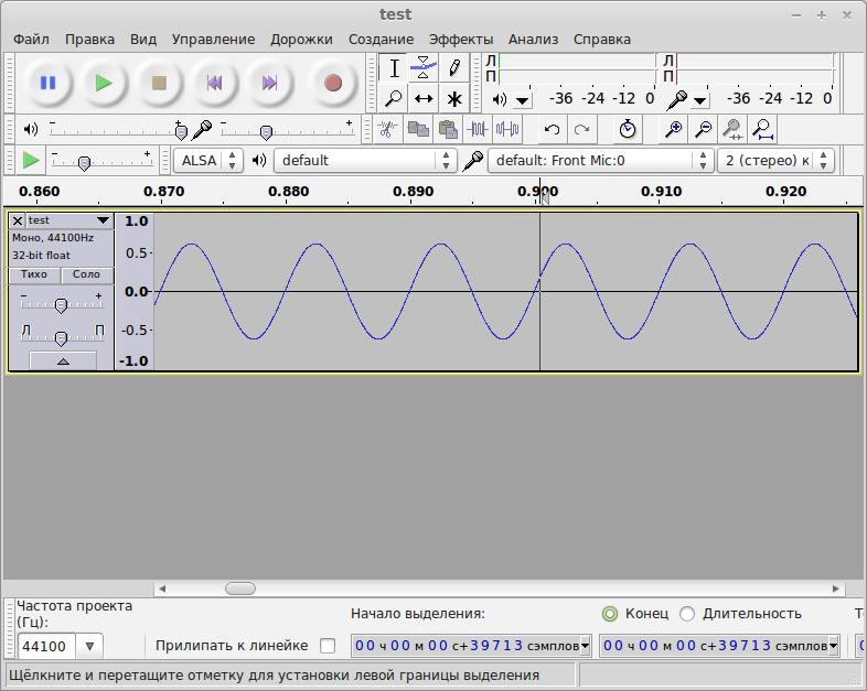
As a result, we get the following file (you can even listen to it with any sound reproducing program). Open this audacity file and see that the signal graph actually corresponds to the pure sine:
Pure tube sinus
Let's look at the spectrum of this sine (Analysis-> Plot spectrum)
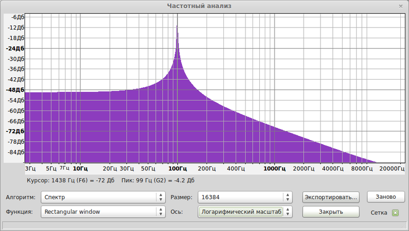
Spectrum spectrum
A clear peak is seen at 100 Hz (logarithmic scale). What is a spectrum? This is the amplitude-frequency response. There is also a phase response characteristic. If you remember, I said above that to build a signal you need to know its frequency, amplitude and phase? So, you can get these parameters from the signal. In this case, we have a graph of frequency amplitude correspondences, with what the amplitude is not in real units, but in decibels.

The value, expressed in decibels , is numerically equal to the decimal logarithm of the dimensionless ratio of a physical quantity to a physical quantity of the same name, taken as the original, multiplied by ten.
In this case, simply the amplitude logarithm multiplied by 10. It is convenient to use the logarithmic scale when working with signals.
I honestly don’t really like the spectrum analyzer in this program, so I decided to write my ownwith blackjack and whores , especially since it’s not hard.
It can be boring here, so you can go directly to the next chapter.
Since I understand perfectly well that it makes no sense to place code wrappers here, those who are really interested in - will find and dig up themselves, and those who are not interested will be bored, I will focus only on the main points of writing a spectrum analyzer wav-file.
First, we need to read the wav file. There it is necessary to read the header in order to understand what the file contains. I did not realize the sea of options for reading this file, and stopped at only one. An example of reading a file was taken from here with almost no changes, IMHO is a great example. There is also a python implementation.
The next thing we need is a fast Fourier transform. This is the same transformation that allows you to get a vector of original signals from a finite set of points. Let it not scare you yet, then I will explain.
Again, the bike did not reinvent, and took a ready-made example from here .
I understand that in order to explain how the program works, it is necessary to explain what the fast Fourier transform is, and this is at least for another non-acidic article.
To begin with, let's arrays arrays:
Let me just say that in the program we read the data into an array of length size_array (which we take from the header of the wav file).
The array for the fast Fourier transform should be a sequence {re [0], im [0], re [1], im [1], ... re [fft_size-1], im [fft_size-1]}, where fft_size = 1 << p is the number of FFT points. I explain in normal language:
This is an array of complex numbers. I’m even afraid to imagine where the complex Fourier transform is used, but in our case the imaginary part is zero and the real part is equal to the value of each point of the array.
Another feature of the fast Fourier transform is that it cheats arrays that are multiples of powers of two only. As a result, we must calculate the minimum power of two:
The logarithm of the number of bytes in the data, divided by the number of bytes at one point.
After that, we consider the turning factors:
And we feed our read array into a Fourier transducer:
At the output we get complex numbers of the form {re [0], im [0], re [1], im [1], ... re [fft_size-1], im [fft_size-1]}. For those who do not know what a complex number is, I will explain. It was not for nothing that I started this article with a heap of rotating vectors and a heap of gifs. So, the vector on the complex plane is determined by the real coordinate a1 and imaginary coordinate a2. Or the length (this is the amplitude Am) and the Psi angle (phase).
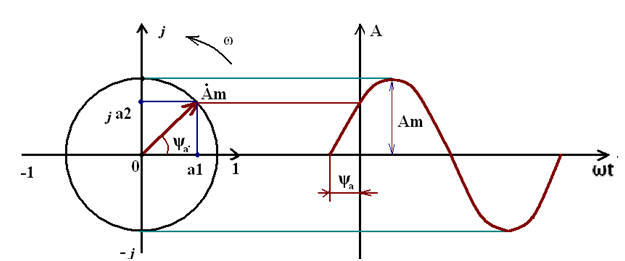
Vector on the complex plane
Please note that size_array = 2 ^ p2. The first point of the array corresponds to the frequency of 0 Hz (constant), the last point corresponds to the sampling frequency, namely 44100 Hz. As a result, we must calculate the frequency corresponding to each point, which will differ by the delta frequency:
Block an array of amplitudes:
And look at the picture: the amplitude is the length of the vector. And we have its projections on the real and imaginary axis. As a result, we will have a right triangle, and here we recall the Pythagorean theorem, and consider the length of each vector, and immediately write it into a text file:
As a result, we obtain a file of the following form:
The final version of the program lives on a githaba here:
github.com/dlinyj/fft
Now we feed the resulting program that sine sound file.
And we get a text file response. We build his schedule with the help of a nest
Script to build:
Pay attention to the restriction in the script on the number of points in X: set xrange [1: 22050]. The sampling frequency is 44100, and if we recall Kotelnikov's theorem, the signal frequency cannot be higher than half the sampling frequency, therefore the signal above 22050 Hz does not interest us. Why so, I advise you to read in the special literature.
So (drum roll), run the script and see:
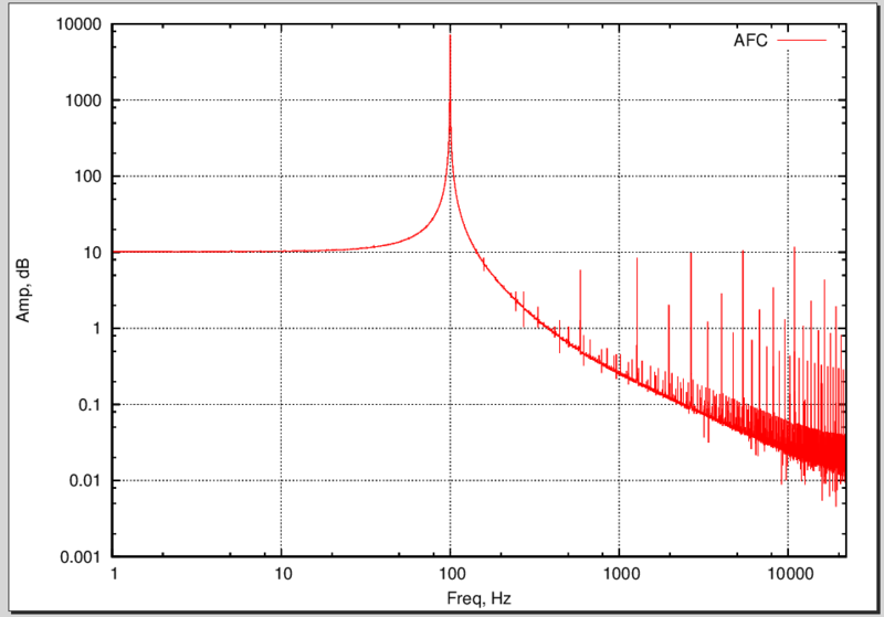
Our signal spectrum
Note the sharp peak at 100 Hz. Do not forget that the axes - the logarithmic scale! The wool on the right, I think, is the Fourier transform error (windows come to mind here).
And let's Let's look at the spectra of other signals!
To begin with, let's build a noise spectrum. The topic of noise, random signals, etc. worthy of a separate course. But we touch it slightly. We modify our program for generating a wav file, add one procedure:
it will generate a random number in the specified range. As a result, main will look like this:
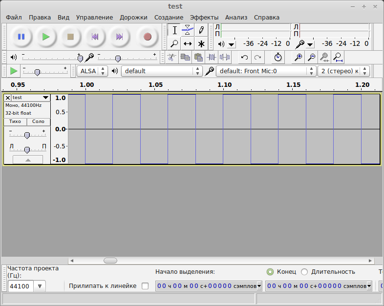
Generate a file (I recommend for listening). Let's look at it in audacity.
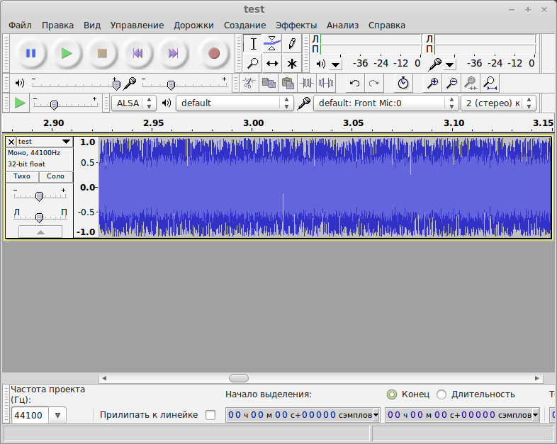
Signal in audacity
Let's look at the spectrum in the program audacity.

Spectrum
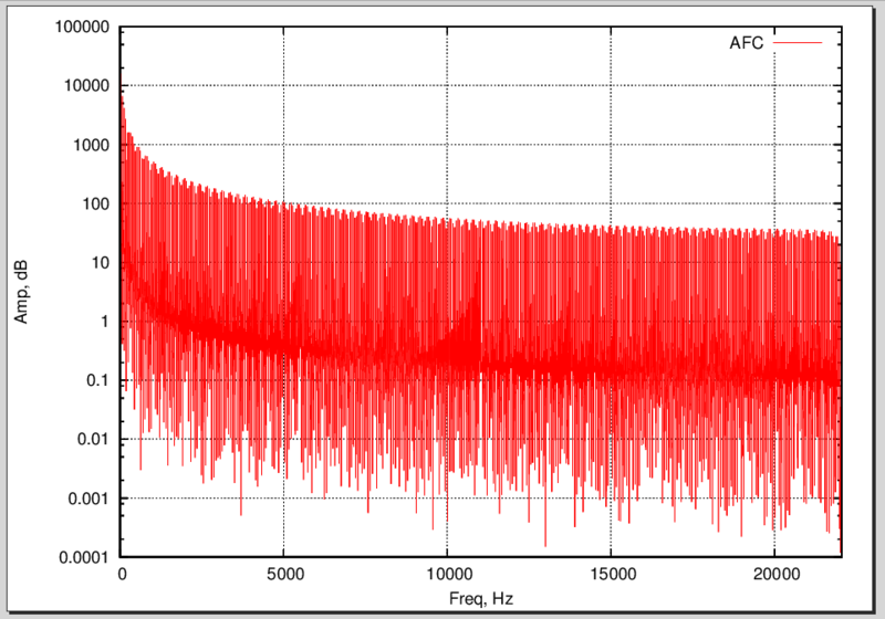
And let's see the spectrum using our program:

Our range
I want to draw attention to a very interesting fact and a feature of noise - it contains the spectra of all harmonics. As can be seen from the graph, the spectrum is quite even. White noise is usually used for frequency analysis of bandwidth, for example, audio equipment. There are other types of noise: pink, blue and others . Homework - find out how they differ.
And now let's see another interesting signal - the meander. There I gave a label above the decomposition of various signals into the Fourier series, you look at how the meander unfolds, write down on a piece of paper, and we will continue.
To generate a meander with a frequency of 25 Hz, we modify our wav-file generator once again:
As a result, we get a sound file (again, I advise you to listen), which you should immediately see in audacity
His majesty is a meander or a meander of a healthy person
We will not languish and look at its spectrum:
Spectrum of meander
So far, it’s not very clear what it is ... And let's see the first few harmonics:

First harmonics
It is quite another matter! Well, let's see the tablet. Look, we only have 1, 3, 5, etc., i.e. odd harmonics. We just see that we have the first harmonic of 25 Hz, the next (third) 75 Hz, then 125 Hz, etc., while the amplitude gradually decreases. The theory has come together with practice!
And now attention! In real life, the meander signal has an infinite amount of harmonics of higher and higher frequency, but as a rule, real electrical circuits cannot pass frequencies higher than a certain frequency (due to inductance and capacitance of the tracks). As a result, you can often see the following signal on the oscilloscope screen:

Meander smoker
This picture is just like a picture from Wikipedia , where not all frequencies are taken as an example of a meander, but only the first few.

The sum of the first harmonics, and how the signal changes
The meander is also actively used in radio engineering (I must say that it is the basis of all digital technology), and it should be understood that with long circuits it can be filtered out so that the native mother does not recognize. It is also used to check the frequency response of various devices. Another interesting fact is that jammers of televisions worked precisely according to the principle of higher harmonics, when the microcircuit itself generated a square wave of tens of MHz, and its higher harmonics could have frequencies of hundreds of MHz, just at the frequency of the television, and the higher harmonics successfully jammed the television's broadcast signal.
In general, the theme of such experiments is endless, and you can now continue it yourself.

Book
For those who do not understand what we are doing here, or vice versa, for those who understand, but want to understand even better, as well as for students studying DSP, I highly recommend this book. This is the DSP for dummies, which is the author of this post. There accessible even for the child language tells the most complex concepts.
In conclusion, I want to say that mathematics is the queen of sciences, but without real use, many people lose interest in it. I hope this post will spur you to the study of such a wonderful subject as signal processing, and in general analog circuitry (plug your ears so that your brains do not flow!). :)
Good luck!
Frequency response noise.
Personally, after reading these articles (for example, this one ) I didn’t understand what it was and why it was needed in real life, although it was interesting and beautiful.
It would be desirable not just to look at beautiful pictures, but to say so, to feel in your gut, what and how it works. And I will give a concrete example with the generation and processing of sound files. It will be possible to listen to the sound and look at its spectrum, and understand why this is so.
The article will not be of interest to those who own the theory of functions of a complex variable, DSP, and other terrible topics. It is more likely for the curious, schoolchildren, students and their sympathizers :).
')
Immediately make a reservation, I am not a mathematician, and I can even say many things incorrectly (correct with a personal message), and I am writing this article based on my own experience and my own understanding of current processes. If you are ready, then go.
A few words about the materiel
If we recall a school course in mathematics, then we used a circle to build a sine graph. In general, it turns out that the rotational motion can be turned into a sinusoid (like any harmonic oscillation). The best illustration of this process is given in wikipedia.
Harmonic vibrations
Those. in fact, the sine plot is obtained from the rotation of the vector, which is described by the formula:
f(x) = A sin (ωt + φ),where A is the vector length (amplitude of oscillations), φ is the initial angle (phase) of the vector at time zero, ω is the angular velocity of rotation, which is equal to:
ω = 2 πf, where f is the frequency in Hertz.
As we can see, knowing the signal frequency, amplitude and angle, we can build a harmonic signal.
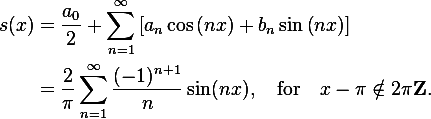
Magic begins when it turns out that the representation of absolutely any signal can be represented as a sum (often infinite) of various sinusoids. In other words, in the form of a Fourier series.
I will give an example from the English Wikipedia . For example, take a ramp.
Ramp
Its sum will be represented by the following formula:
If we successively sum up, take n = 1 first, then n = 2, etc., we will see how our harmonic sinusoidal signal gradually turns into a saw:
Probably the most beautiful thing is illustrated by one program I found in the open spaces of the network. It was already mentioned above that the sine graph is a projection of a rotating vector, but what about more complex signals? This, oddly enough, the projection of a set of rotating vectors, or rather their sum, and it looks like this:
Vectors draw a saw.
In general, I recommend to go by the link and try to play with the parameters, and see how the signal changes. IMHO more visual toys for understanding, I have not yet met.
It should also be noted that there is an inverse procedure that allows to obtain from this signal the frequency, amplitude and initial phase (angle), which is called the Fourier Transform.
Fourier series decomposition of some known periodic functions ( from here )
I will not dwell on it in detail, but I will show how this can be applied in life. In the list of references I will recommend something where you can read more about the materiel.
We turn to practical exercises!
It seems to me that each student wonders, sitting at a lecture, for example, on matan: why do I need all this nonsense? And as a rule, not finding an answer in the foreseeable future, unfortunately, loses interest in the subject. Therefore, I will immediately show the practical application of this knowledge, and you will already master this knowledge yourself :).
All further I will implement on it. I did everything, of course, under Linux, but I didn’t use any specifics; in theory, the program will compile and work under other platforms.
To begin with we will write the program for formation of the sound file. Wav file was taken as the easiest. Read about its structure here .
In short, the structure of the wav file is described as follows: the header, which describes the file format, and then (in our case) an array of 16-bit data (pointed) length: sampling frequency * t seconds or 44100 * t pieces.
An example was taken here to generate a sound file. I modified it a bit, corrected the errors, and the final version with my edits now lies on the github here
github.com/dlinyj/generate_wav
We will generate a two-second sound file with a pure sine with a frequency of 100 Hz. To do this, modify the program as follows:
#define S_RATE (44100) // #define BUF_SIZE (S_RATE*10) /* 2 second buffer */ …. int main(int argc, char * argv[]) { ... float amplitude = 32000; // float freq_Hz = 100; // /* fill buffer with a sine wave */ for (i=0; i<BUF_SIZE; i++) { buffer[i] +=(int)(amplitude * sin((float)(2*M_PI*i*freq_Hz/S_RATE))); } write_wav("test.wav", BUF_SIZE, buffer, S_RATE); return 0; } I pay attention that the formula of pure sine corresponds to that about which we spoke above. The amplitude of 32,000 (it was possible to take 32767) corresponds to a value that can take a 16-bit number (from minus 32767 to plus 32767).
As a result, we get the following file (you can even listen to it with any sound reproducing program). Open this audacity file and see that the signal graph actually corresponds to the pure sine:
Pure tube sinus
Let's look at the spectrum of this sine (Analysis-> Plot spectrum)
Spectrum spectrum
A clear peak is seen at 100 Hz (logarithmic scale). What is a spectrum? This is the amplitude-frequency response. There is also a phase response characteristic. If you remember, I said above that to build a signal you need to know its frequency, amplitude and phase? So, you can get these parameters from the signal. In this case, we have a graph of frequency amplitude correspondences, with what the amplitude is not in real units, but in decibels.
The value, expressed in decibels , is numerically equal to the decimal logarithm of the dimensionless ratio of a physical quantity to a physical quantity of the same name, taken as the original, multiplied by ten.
In this case, simply the amplitude logarithm multiplied by 10. It is convenient to use the logarithmic scale when working with signals.
I honestly don’t really like the spectrum analyzer in this program, so I decided to write my own
We write your spectrum analyzer
It can be boring here, so you can go directly to the next chapter.
Since I understand perfectly well that it makes no sense to place code wrappers here, those who are really interested in - will find and dig up themselves, and those who are not interested will be bored, I will focus only on the main points of writing a spectrum analyzer wav-file.
First, we need to read the wav file. There it is necessary to read the header in order to understand what the file contains. I did not realize the sea of options for reading this file, and stopped at only one. An example of reading a file was taken from here with almost no changes, IMHO is a great example. There is also a python implementation.
The next thing we need is a fast Fourier transform. This is the same transformation that allows you to get a vector of original signals from a finite set of points. Let it not scare you yet, then I will explain.
Again, the bike did not reinvent, and took a ready-made example from here .
I understand that in order to explain how the program works, it is necessary to explain what the fast Fourier transform is, and this is at least for another non-acidic article.
To begin with, let's arrays arrays:
c = calloc(size_array*2, sizeof(float)); // in = calloc(size_array*2, sizeof(float)); // out = calloc(size_array*2, sizeof(float)); // Let me just say that in the program we read the data into an array of length size_array (which we take from the header of the wav file).
while( fread(&value,sizeof(value),1,wav) ) { in[j]=(float)value; j+=2; if (j > 2*size_array) break; } The array for the fast Fourier transform should be a sequence {re [0], im [0], re [1], im [1], ... re [fft_size-1], im [fft_size-1]}, where fft_size = 1 << p is the number of FFT points. I explain in normal language:
This is an array of complex numbers. I’m even afraid to imagine where the complex Fourier transform is used, but in our case the imaginary part is zero and the real part is equal to the value of each point of the array.
Another feature of the fast Fourier transform is that it cheats arrays that are multiples of powers of two only. As a result, we must calculate the minimum power of two:
int p2=(int)(log2(header.bytes_in_data/header.bytes_by_capture)); The logarithm of the number of bytes in the data, divided by the number of bytes at one point.
After that, we consider the turning factors:
fft_make(p2,c);// ( , ). And we feed our read array into a Fourier transducer:
fft_calc(p2, c, in, out, 1); //( , ). At the output we get complex numbers of the form {re [0], im [0], re [1], im [1], ... re [fft_size-1], im [fft_size-1]}. For those who do not know what a complex number is, I will explain. It was not for nothing that I started this article with a heap of rotating vectors and a heap of gifs. So, the vector on the complex plane is determined by the real coordinate a1 and imaginary coordinate a2. Or the length (this is the amplitude Am) and the Psi angle (phase).
Vector on the complex plane
Please note that size_array = 2 ^ p2. The first point of the array corresponds to the frequency of 0 Hz (constant), the last point corresponds to the sampling frequency, namely 44100 Hz. As a result, we must calculate the frequency corresponding to each point, which will differ by the delta frequency:
double delta=((float)header.frequency)/(float)size_array; // . Block an array of amplitudes:
double * ampl; ampl = calloc(size_array*2, sizeof(double)); And look at the picture: the amplitude is the length of the vector. And we have its projections on the real and imaginary axis. As a result, we will have a right triangle, and here we recall the Pythagorean theorem, and consider the length of each vector, and immediately write it into a text file:
for(i=0;i<(size_array);i+=2) { fprintf(logfile,"%.6f %f\n",cur_freq, (sqrt(out[i]*out[i]+out[i+1]*out[i+1]))); cur_freq+=delta; } As a result, we obtain a file of the following form:
… 11.439514 10.943008 11.607742 56.649738 11.775970 15.652428 11.944199 21.872342 12.112427 30.635371 12.280655 30.329171 12.448883 11.932371 12.617111 20.777617 ... The final version of the program lives on a githaba here:
github.com/dlinyj/fft
We try!
Now we feed the resulting program that sine sound file.
./fft_an ../generate_wav/sin\ 100\ Hz.wav format: 16 bits, PCM uncompressed, channel 1, freq 44100, 88200 bytes per sec, 2 bytes by capture, 2 bits per sample, 882000 bytes in data chunk=441000 log2=18 size array=262144 wav format Max Freq = 99.928 , amp =7216.136 And we get a text file response. We build his schedule with the help of a nest
Script to build:
#! /usr/bin/gnuplot -persist set terminal postscript eps enhanced color solid set output "result.ps" #set terminal png size 800, 600 #set output "result.png" set grid xtics ytics set log xy set xlabel "Freq, Hz" set ylabel "Amp, dB" set xrange [1:22050] #set yrange [0.00001:100000] plot "test.txt" using 1:2 title "AFC" with lines linestyle 1 Pay attention to the restriction in the script on the number of points in X: set xrange [1: 22050]. The sampling frequency is 44100, and if we recall Kotelnikov's theorem, the signal frequency cannot be higher than half the sampling frequency, therefore the signal above 22050 Hz does not interest us. Why so, I advise you to read in the special literature.
So (drum roll), run the script and see:
Our signal spectrum
Note the sharp peak at 100 Hz. Do not forget that the axes - the logarithmic scale! The wool on the right, I think, is the Fourier transform error (windows come to mind here).
And let's pamper?
And let's Let's look at the spectra of other signals!
Around the noise ...
To begin with, let's build a noise spectrum. The topic of noise, random signals, etc. worthy of a separate course. But we touch it slightly. We modify our program for generating a wav file, add one procedure:
double d_random(double min, double max) { return min + (max - min) / RAND_MAX * rand(); } it will generate a random number in the specified range. As a result, main will look like this:
int main(int argc, char * argv[]) { int i; float amplitude = 32000; srand((unsigned int)time(0)); // for (i=0; i<BUF_SIZE; i++) { buffer[i] +=(int)amplitude*d_random(-1.0, 1.0); //nois } write_wav("test.wav", BUF_SIZE, buffer, S_RATE); return 0; } Generate a file (I recommend for listening). Let's look at it in audacity.
Signal in audacity
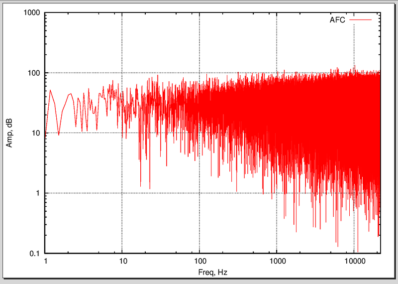
Let's look at the spectrum in the program audacity.
Spectrum
And let's see the spectrum using our program:
Our range
I want to draw attention to a very interesting fact and a feature of noise - it contains the spectra of all harmonics. As can be seen from the graph, the spectrum is quite even. White noise is usually used for frequency analysis of bandwidth, for example, audio equipment. There are other types of noise: pink, blue and others . Homework - find out how they differ.
And compote?
And now let's see another interesting signal - the meander. There I gave a label above the decomposition of various signals into the Fourier series, you look at how the meander unfolds, write down on a piece of paper, and we will continue.
To generate a meander with a frequency of 25 Hz, we modify our wav-file generator once again:
int main(int argc, char * argv[]) { int i; short int meandr_value=32767; /* fill buffer with a sine wave */ for (i=0; i<BUF_SIZE; i++) { //meandr if (!(i%(S_RATE/((int)freq_Hz/2)))) { if (meandr_value==32767) { meandr_value=-32767; } else { meandr_value=32767; } } buffer[i]=meandr_value; } write_wav("test.wav", BUF_SIZE, buffer, S_RATE); return 0; } As a result, we get a sound file (again, I advise you to listen), which you should immediately see in audacity
His majesty is a meander or a meander of a healthy person
We will not languish and look at its spectrum:
Spectrum of meander
So far, it’s not very clear what it is ... And let's see the first few harmonics:
First harmonics
It is quite another matter! Well, let's see the tablet. Look, we only have 1, 3, 5, etc., i.e. odd harmonics. We just see that we have the first harmonic of 25 Hz, the next (third) 75 Hz, then 125 Hz, etc., while the amplitude gradually decreases. The theory has come together with practice!
And now attention! In real life, the meander signal has an infinite amount of harmonics of higher and higher frequency, but as a rule, real electrical circuits cannot pass frequencies higher than a certain frequency (due to inductance and capacitance of the tracks). As a result, you can often see the following signal on the oscilloscope screen:
Meander smoker
This picture is just like a picture from Wikipedia , where not all frequencies are taken as an example of a meander, but only the first few.
The sum of the first harmonics, and how the signal changes
The meander is also actively used in radio engineering (I must say that it is the basis of all digital technology), and it should be understood that with long circuits it can be filtered out so that the native mother does not recognize. It is also used to check the frequency response of various devices. Another interesting fact is that jammers of televisions worked precisely according to the principle of higher harmonics, when the microcircuit itself generated a square wave of tens of MHz, and its higher harmonics could have frequencies of hundreds of MHz, just at the frequency of the television, and the higher harmonics successfully jammed the television's broadcast signal.
In general, the theme of such experiments is endless, and you can now continue it yourself.
Recommendations for reading
Book
For those who do not understand what we are doing here, or vice versa, for those who understand, but want to understand even better, as well as for students studying DSP, I highly recommend this book. This is the DSP for dummies, which is the author of this post. There accessible even for the child language tells the most complex concepts.
Conclusion
In conclusion, I want to say that mathematics is the queen of sciences, but without real use, many people lose interest in it. I hope this post will spur you to the study of such a wonderful subject as signal processing, and in general analog circuitry (plug your ears so that your brains do not flow!). :)
Good luck!
Source: https://habr.com/ru/post/219337/
All Articles