Identification of fast thermal processes
Recently, I managed to complete some of the work on a very interesting project at the Institute of Physics and Technology. Ioffe and get enough experimental data to share with you.
Physics from St. Petersburg Physicotechnical Institute to them. Ioffe is engaged in growing nitride gallium semiconductor structures, which have good indicators of the velocity of charge carriers during the transition and a large coefficient of thermal conductivity. The process of growth of such a structure takes place at a temperature of 1000 C (1273 K) and atmospheric pressure. Everything happens in a special chamber located in a sealed area. When the structure is grown, the entire volume of the reactor and the hermetic zone is filled with nitrogen. As the structure grows, the substrate holder rotates at a rate of once per second. Such operations relate to rapid thermal processes, the rate of temperature change in which varies from several units to hundreds of degrees per second.
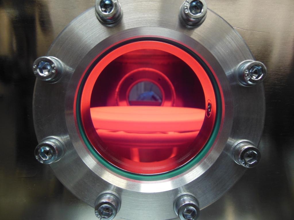
My task was to control the temperature of the graphite substrate holder using inductive heating.
Technical specifications of the installation are as follows. To measure the temperature, a laser pyrometer is used, which takes data in the center of graphite. The frequency of information retrieval 10 times per second, the measurement step is 1 degree. The value of power transmitted to graphite relies directly proportional to the power at the inductor. The generator control inductor has a digital output, which transmitted the values of voltage, current and power.
To begin with, it was necessary to adjust the temperature regulator so that in the process of growth there were no strong fluctuations. We coped with this task rather quickly, but our solution gave a qualitative result only at high temperatures. For other processes required to change the coefficients.
Since this work fit into the theme of my candidate, I wanted to write some tricky control algorithm based on the analysis of the model of thermal processes. To begin with, I got acquainted with the law of Stefan - Boltzmann , the radiation power of an absolutely black body is directly proportional to the surface area and the fourth power of the temperature. Taking convection into account, we can write the equation for thermal processes at the point of temperature removal

where T is the temperature, P is the power, Tc is the temperature of the surrounding objects that heat graphite with its own radiation, Ta is the gas temperature near the pickup point, which performs convection, B, A1, A2 are the coefficients that must be identified. For simplicity, let's replace all the components of the equation, which we can consider constant in the steady state process and we will consider the following equation

Now we have at our disposal a model from which we can push off with further data analysis. In the experiment, a meander was applied as a signal.


If we obtain an estimate of the velocity of temperature, then it will be possible to create a regression model with known temperature and power of the control inductor, and calculate the coefficients in the equation.
I have been using Scilab for quite some time and this time I decided not to change myself. For this task, I chose to take a derivative in the Fourier image. But to start working with real data, you need to interpol measurements to obtain a uniform time axis.
It should be noted that the variable "int_temp_diff" will contain the speed data, but they look very unacceptable.

So let's move on to working with data in the Fourier image. We will need to increase the additional data tail, so that there is no gap at the end, mirroring the temperature data graph.

Then we set the frequency axis and make a discrete Fourier transform.


At a frequency of 1 hertz, a clear peak is visible, this is due to the fact that the substrate holder rotates with this frequency. Other frequencies have broken through due to the fact that graphite is heated unevenly, and during rotation the temperature may increase and decrease several times.
To take the derivative in the Fourier image, simply multiply by . After this, we do the inverse Fourier transform.

This is of course a little better than what the function returns, taking a derivative via cubic splines, but identification with this yields poor-quality results. We have to resort to filtering the signal.
On the advice of my friend Jura, who is setting up ship control systems, it was decided to use the Blackman-Harris window to cut out the extra frequencies. Since in the process of growth graphite rotates with a frequency of 1 time per second, all vibrations with a frequency higher than this are not interesting for us. Therefore, it is worth cutting out all vibrations above 1 [Hz]:

It became much better. With this we proceed to the calculation of the regression coefficients.
To get good data, you must first normalize the data vectors. For a free constant in the equation, you need to specify a vector filled with units.
Now you can begin to find the values of the constants. We make a matrix containing the values of three variables and constants. With this, we divide each of the data vectors by its length. To obtain the coefficients, you need to multiply the pseudo-inverse matrix by the normalized vector of data of the rate of temperature change.
And after that it is necessary to return to the original values of the coefficient vector.
As a result, the following values were obtained: a0 = [- 1.073D-12, - 0.0029096, 0.0004617, 2.0969723], which is close enough to the result of our foreign colleagues , although they use tube heating.
Now you can begin to check the results on the resulting model. We use for this the virtual simulation package Xcos Scilab. Since we have a differential equation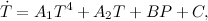 , describing the thermal process in the reactor, and all the coefficients to it, then we collect the following scheme.

Using the “From Workspace” block, we submit experimental power data, first creating the structure V for this block. Set the sampling frequency and time to start the simulation in the “Clock” block. The length of the output data structure is set equal to the input. The final simulation time should be equal to the experiment time. Compiled model run in the text of the program and compare the graphs of the experiment and simulation.


Here is the same thing, but for harmonic disturbances with varying frequency.


Many thanks to the supervisor of Arastas for their invaluable help and participation in the preparation of the material. I thank Evgeny Zavarin for providing access to the installation and software implementation of all experiments.
Physics from St. Petersburg Physicotechnical Institute to them. Ioffe is engaged in growing nitride gallium semiconductor structures, which have good indicators of the velocity of charge carriers during the transition and a large coefficient of thermal conductivity. The process of growth of such a structure takes place at a temperature of 1000 C (1273 K) and atmospheric pressure. Everything happens in a special chamber located in a sealed area. When the structure is grown, the entire volume of the reactor and the hermetic zone is filled with nitrogen. As the structure grows, the substrate holder rotates at a rate of once per second. Such operations relate to rapid thermal processes, the rate of temperature change in which varies from several units to hundreds of degrees per second.
My task was to control the temperature of the graphite substrate holder using inductive heating.
Technical specifications of the installation are as follows. To measure the temperature, a laser pyrometer is used, which takes data in the center of graphite. The frequency of information retrieval 10 times per second, the measurement step is 1 degree. The value of power transmitted to graphite relies directly proportional to the power at the inductor. The generator control inductor has a digital output, which transmitted the values of voltage, current and power.
To begin with, it was necessary to adjust the temperature regulator so that in the process of growth there were no strong fluctuations. We coped with this task rather quickly, but our solution gave a qualitative result only at high temperatures. For other processes required to change the coefficients.
Since this work fit into the theme of my candidate, I wanted to write some tricky control algorithm based on the analysis of the model of thermal processes. To begin with, I got acquainted with the law of Stefan - Boltzmann , the radiation power of an absolutely black body is directly proportional to the surface area and the fourth power of the temperature. Taking convection into account, we can write the equation for thermal processes at the point of temperature removal
where T is the temperature, P is the power, Tc is the temperature of the surrounding objects that heat graphite with its own radiation, Ta is the gas temperature near the pickup point, which performs convection, B, A1, A2 are the coefficients that must be identified. For simplicity, let's replace all the components of the equation, which we can consider constant in the steady state process and we will consider the following equation
Now we have at our disposal a model from which we can push off with further data analysis. In the experiment, a meander was applied as a signal.
If we obtain an estimate of the velocity of temperature, then it will be possible to create a regression model with known temperature and power of the control inductor, and calculate the coefficients in the equation.
I have been using Scilab for quite some time and this time I decided not to change myself. For this task, I chose to take a derivative in the Fourier image. But to start working with real data, you need to interpol measurements to obtain a uniform time axis.
xx = linspace(0, round(time($)), round(time($))*fs+1)'; //New time axes' d=splin(time,temp,"monotone"); [int_temp,int_temp_diff] = interp(xx, time, temp, d); It should be noted that the variable "int_temp_diff" will contain the speed data, but they look very unacceptable.
So let's move on to working with data in the Fourier image. We will need to increase the additional data tail, so that there is no gap at the end, mirroring the temperature data graph.
Then we set the frequency axis and make a discrete Fourier transform.
fs = 10; //Sample frequency in = [int_temp;int_temp($:-1:1)]; N = length ( in ); frequency = [0 : (N-1)] / N * fs; frequency (N/2+1 : $) = frequency (N/2+1 : $) -fs; frequency = frequency'; sp = fft(in); //Fast Fourier Transform At a frequency of 1 hertz, a clear peak is visible, this is due to the fact that the substrate holder rotates with this frequency. Other frequencies have broken through due to the fact that graphite is heated unevenly, and during rotation the temperature may increase and decrease several times.
To take the derivative in the Fourier image, simply multiply by
. After this, we do the inverse Fourier transform. omega = (2*%pi*%i*frequency); tmp = sp.*omega; out = real(fft(tmp,1)); speed_temp = out(1:N/2); This is of course a little better than what the function returns, taking a derivative via cubic splines, but identification with this yields poor-quality results. We have to resort to filtering the signal.
On the advice of my friend Jura, who is setting up ship control systems, it was decided to use the Blackman-Harris window to cut out the extra frequencies. Since in the process of growth graphite rotates with a frequency of 1 time per second, all vibrations with a frequency higher than this are not interesting for us. Therefore, it is worth cutting out all vibrations above 1 [Hz]:
cf = 1; //Cutoff frequency k = round(cf*N/fs); L = 2*k+1; a0=0.35875; a1=0.48829; a2=0.14128; a3=0.01168; for j=0:L-1, w(j+1) = a0 - a1*cos(2*%pi*j/(L-1))+a2*cos(4*%pi*j/(L-1))-a3*cos(6*%pi*j/(L-1)); end h = zeros(frequency); for j=1:1:k+1 h(j) = w(k+j); end h([$:-1:$-k]) = h([1:1:k+1]); omega = (2*%pi*%i*frequency); omega = omega.*h; tmp = sp.*omega; out = real(fft(tmp,1)); speed_temp = out(1:N/2); It became much better. With this we proceed to the calculation of the regression coefficients.
To get good data, you must first normalize the data vectors. For a free constant in the equation, you need to specify a vector filled with units.
constant (1:length(int_power)) = 1; norm_4_temp = norm( int_temp.^4 ); norm_int_temp = norm( int_temp ); norm_int_power = norm( int_power ); norm_speed_temp = norm( speed_temp ); norm_constant = norm( constant ); Now you can begin to find the values of the constants. We make a matrix containing the values of three variables and constants. With this, we divide each of the data vectors by its length. To obtain the coefficients, you need to multiply the pseudo-inverse matrix by the normalized vector of data of the rate of temperature change.
LSM = [ int_temp.^4/norm_4_temp , int_temp/norm_int_temp , int_power/norm_int_power , constant/norm_constant ] ; a0 = pinv(LSM) * speed_temp / norm_speed_temp ; And after that it is necessary to return to the original values of the coefficient vector.
a0(1) = a0(1)*norm_speed_temp/norm_4_temp; a0(2) = a0(2)*norm_speed_temp/norm_int_temp; a0(3) = a0(3)*norm_speed_temp/norm_int_power; a0(4) = a0(4)*norm_speed_temp/norm_constant; As a result, the following values were obtained: a0 = [- 1.073D-12, - 0.0029096, 0.0004617, 2.0969723], which is close enough to the result of our foreign colleagues , although they use tube heating.
Now you can begin to check the results on the resulting model. We use for this the virtual simulation package Xcos Scilab. Since we have a differential equation
, describing the thermal process in the reactor, and all the coefficients to it, then we collect the following scheme.Using the “From Workspace” block, we submit experimental power data, first creating the structure V for this block. Set the sampling frequency and time to start the simulation in the “Clock” block. The length of the output data structure is set equal to the input. The final simulation time should be equal to the experiment time. Compiled model run in the text of the program and compare the graphs of the experiment and simulation.
V.time = xx; V.values = int_power; importXcosDiagram("D:\PhD\Term_model.zcos"); xcos_simulate(scs_m,4); plot(time,temp); plot(A.time,A.values,"r--"); Here is the same thing, but for harmonic disturbances with varying frequency.
Many thanks to the supervisor of Arastas for their invaluable help and participation in the preparation of the material. I thank Evgeny Zavarin for providing access to the installation and software implementation of all experiments.
')
Source: https://habr.com/ru/post/218297/
All Articles