Analysis and visualization of real tabular data in R

The material will be useful to those who master the R language as a tool for analyzing tabular data and want to see a cross-cutting example of the implementation of the main processing steps.
Below is a demonstration of loading data from csv files, parsing text strings with data cleansing elements, aggregating data by analytic measurements, and plotting diagrams.
The example actively uses the functionality of the data.table, reshape2, stringdist, and ggplot2 packages.

Information on the issued permits for carrying out passenger and baggage passenger taxi services in Moscow was taken as “real data”. The data is provided for general use by the Department of Transport and the development of road and transport infrastructure of the city of Moscow. Page data set data.mos.ru/datasets/655
The source data has the following format:

ROWNUM;VEHICLE_NUM;FULL_NAME;BLANK_NUM;VEHICLE_BRAND_MODEL;INN;OGRN 1;"248197";" «-»";"017263";"FORD FOCUS";"7734653292";"1117746207578" 2;"249197";" «-»";"017264";"FORD FOCUS";"7734653292";"1117746207578" 3;"245197";" «-»";"017265";"FORD FOCUS";"7734653292";"1117746207578" ```

1. Download primary data

Data can be downloaded directly from the site. In the boot process, we immediately rename the columns conveniently.

 url <- "http://data.mos.ru/datasets/download/655" colnames = c("RowNumber", "RegPlate", "LegalName", "DocNum", "Car", "INN", "OGRN", "Void") rawdata <- read.table(url, header = TRUE, sep = ";", colClasses = c("numeric", rep("character",6), NA), col.names = colnames, strip.white = TRUE, blank.lines.skip = TRUE, stringsAsFactors = FALSE, encoding = "UTF-8")

Now you can begin to analyze and visualize ...

2. Data Conversion

Suppose that it is necessary to analyze the distribution of the number of cars registered as taxis, depending on the organizational form of the licensee and the make of the car. The relevant data is not highlighted separately, but all the necessary information is contained in the fields FULL_NAME (renamed LegalName) and VEHICLE_BRAND_MODEL (Car).
In the process of converting the original data is necessary

from the LegalName field to separate the organizational and legal form into a separate OrgType field;
from the Car field, select the car brand in a separate CarBrand field;
discard unused fields.

For simplicity, we assume that the first words of the LegalName and Car fields are, respectively, the organizational and legal form and the make of the car (below it will be clear what to do with the exceptions). Unnecessary fields will be discarded automatically during the process of converting data.frame to data.table with explicit indication of the list of portable fields.

 ptn <- "^(.+?) (.+)$" # regexp pattern to match first word dt <- data.table(rawdata)[, list(RegPlate, LegalName, Car, OGRN, OrgType = gsub(ptn, "\\1" , toupper( LegalName )), CarBrand = gsub(ptn, "\\1", toupper( Car ))) ] rm(rawdata) # Clear some memory

3. First results

Check what organizational forms were selected from the data.

 sort( table(dt$OrgType) )

 ##      ## 1 392 649 17118 17680

The data is formed quite correctly: individual entrepreneurs are leading in terms of the number of licenses obtained (reducing the tax burden?), There are limited liability companies, open and closed joint-stock companies, and even one non-commercial partnership.
In order to determine how many independent licensees (and not cars) have received a license, depending on the legal form, it is necessary to sum over the field that uniquely characterizes the legal entity (OGRN).

 dt[, list( N = length( unique(OGRN) ) ), by = OrgType][order(N, decreasing = TRUE)]

 ## OrgType N ## 1:  12352 ## 2:  563 ## 3:  14 ## 4:  6 ## 5:  1

Data cleansing

What brands of cars are used as a taxi in Moscow?
There are quite a few car brands represented in the data set: 115, but are they really all unique? For example, we deduce all marks starting with the letter “M”.

 sort( unique( dt[grep("^M.*", CarBrand), CarBrand]))

 ## [1] "M214" "MASERATI" "MAZDA" ## [4] "MAZDA-" "MERCEDES" "MERCEDES-BENZ" ## [7] "MERCEDES-BENZ-" "MERCEDES-BENZ-S500" "MERCEDES-BENZC" ## [10] "MERCEDES-BENZE200K" "MERCEDES-BENZE220CDI" "MERCEDES-BNZ" ## [13] "MERCERDES-BENZ" "MERCRDES" "MERCRDES-BENZ" ## [16] "MERSEDES-" "MERSEDES-BENZ" "METROCAB" ## [19] "MG" "MINI" "MITSUBISHI"

Unfortunately, a large number of brands of cars is largely due to errors in the data. For example, the same brand - MERCEDES-BENZ - is found under different names. Before analyzing the data must be cleared.
The program basis for clearing textual information is the search function “distance between lines”. For each pair of rows, they compute a metric characterizing the complexity of converting one string to another using letter operations. The more similar the lines, the less operations are required. Ideally, identical lines should have a distance equal to zero, and the most dissimilar ones should be one. This is exactly how the Jaro-Winkler algorithm of the stringdist function of the same package works.
Let's compare several lines, only we will count not distance, but similarity, 1-stringdist.

 1 - stringdist( c("MERCEDES","MERSEDES","MAZDA","RENAULT","SAAB"), "MERCEDES", method = "jw", p = 0.1)

 ## [1] 1.0000 0.9417 0.5950 0.3452 0.0000

At first glance, the task of data cleaning is solved simply: for each record, it suffices to choose the most similar value from the directory. Unfortunately, this approach does not always work. First, the directory may not be (as in the current case). Secondly, some situations require manual data correction, even with an accurate reference guide. For example, from the point of view of the method, three marks are equally suitable as an alternative to the incorrect value of “BAZ”:

 1 - stringdist("BAZ", c("VAZ", "UAZ", "ZAZ"), method = "jw", p = 0.1)

 ## [1] 0.7778 0.7778 0.7778

Below, a semi-automatic correction method is used, which makes it possible to significantly ease the work of a data cleansing specialist by programmatically generating options for corrections with which the analyst can either agree or manually correct.
It is assumed that in a large amount of data with a small number of errors, frequently occurring values are correct, and rarely occurring errors. Frequency values are used as a weighting factor, proportionally increasing the proximity metric of rows. So that frequently encountered brands of cars do not go ahead at the expense of quantity, and not similarity, only metrics of values with a degree of similarity above the threshold value t (about choosing t later) are taken into account. For each possible value of the make of machine, a recommended reference value is thus determined from the same data set. The “brand - proposed fix” pairs are displayed in a csv file. After analysis and corrections, the corrected csv file is loaded and serves as a dictionary.
We start by constructing a function that returns the best match on an existing dataset.

 bestmatch.gen <- function(wc, t = 0){ # wc = counts of all base text words # t = threshold: only the words with similarity above threshold count bestmatch <- function(a){ sim <- 1 - stringdist( toupper(a), toupper( names(wc) ) , method = "jw", p = 0.1 ) # Compute weights and implicitly cut off everything below threshold weights <- sim * wc * (sim > t) # Return the one with maximum combined weight names( sort(weights, decr = TRUE)[1] ) } bestmatch }

The threshold value t chosen empirically. Here is an example of the function for the threshold parameter t = 0.7.

  bm07 <- bestmatch.gen( table( dt$CarBrand), t = 0.7 ) s <- c("FORD","RENO","MERS","PEGO") sapply(s, bm07)

 ## FORD RENO MERS PEGO ## "FORD" "RENAULT" "MERCEDES-BENZ" "PEUGEOT"

At first glance, everything worked wonderfully. However, rejoice too early. Brand names with similar names that are well represented in the data set can “pull over” other correct names.

 s <- c("HONDA", "CHRYSLER", "VOLVO") sapply(s, bm07)

 ## HONDA CHRYSLER VOLVO ## "HYUNDAI" "CHEVROLET" "VOLKSWAGEN"

Let's try to increase the threshold value t.

 bm09 <- bestmatch.gen( table( dt$CarBrand), t = 0.9 ) s <- c("HONDA","CHRYSLER","VOLVO") sapply(s, bm09)

 ## HONDA CHRYSLER VOLVO ## "HONDA" "CHRYSLER" "VOLVO"

Everything is good? Nearly. Too hard clipping of unlike strings causes the algorithm to consider some erroneous values to be correct. Such errors will have to be corrected manually.

 s <- c("CEAT", "CVEVROLET") sapply(s, bm09)

 ## CEAT CVEVROLET ## "CEAT" "CVEVROLET"

Now everything is ready for the formation of a file of the dictionary of unique values of the brands of cars. Since the file will need to be edited by hand, it is convenient if it contains additional fields indicating whether the proposed replacement differs from the original value (this is not always obvious), how often the brand name is found, as well as a label that draws attention to the recording depending on some kind of statistical characteristics of the set. In this case, we want to catch situations in which the algorithm offers infrequent (presumably erroneous) values as correct.

 ncb <- table(dt$CarBrand) scb <- names(ncb) # Source Car Brands acb <- sapply(scb, bm09) # Auto-generated replacement cbdict_out <- data.table(ncb)[,list( SourceName = scb, AutoName = acb, SourceFreq = as.numeric(ncb), AutoFreq = as.numeric( ncb[acb] ), Action = ordered( scb == acb, labels = c("CHANGE","KEEP")), DictName = acb )] # Add alert flag # Alert when suggested is a low-frequency dictionary word cbdict_out <- cbdict_out[, Alert := ordered( AutoFreq <= quantile(AutoFreq, probs = 0.05, na.rm = TRUE), labels = c("GOOD","ALERT")) ] write.table( cbdict_out[ order(SourceName), list( Alert, Action, SourceName, AutoName, SourceFreq, AutoFreq, DictName) ], "cbdict_out.txt", sep = ";", quote = TRUE, col.names = TRUE, row.name = FALSE, fileEncoding = "UTF-8")

You need to check and edit the values of the DictName field and save the file as “cbdict_in.txt” for later download.
The analyzed data set has features that you should pay attention to:

Some lines do not contain the brand of the car - empty or "NO", and some models are difficult to single-identifier: L1H1, M214; manually change to UNKNOWN or similar pseudo-value;
two spellings are equally used: MERCEDES and MERCEDES-BENZ, leaving one, MERCEDES-BENZ;
There are two visually identical independent spellings of ZAZ (in the output there are two lines, and both of the algorithms suggest to save as true, Action = KEEP); apparently, a letter with another UTF-8 code has crept in somewhere;
Some car names do not contain the brand, but only the model: SAMAND (IRAN KHODRO)
confusion with brands TAGAZ - VORTEX and JAC; for simplicity, it is proposed to assign (albeit not quite correctly) the general name TAGAZ to vehicles whose brands were defined as TAGAZ, A21, SUV, SUVT11, VORTEX, JAC.

In addition to the features of the data, there are limitations of the algorithm that need to be corrected manually.

the algorithm suggests some erroneous names as correct alternatives: CEAT, CVEVROLET;
stamps consisting of two words are reduced to one: ALFA (ALFA ROMEO), GREAT (GREAT WALL), IRAN (IRAN KHODRO), LAND (LAND ROVER).

The edited data is loaded from the cbdict_in.txt file.

 if ( file.exists("cbdict_in.txt")) url <- "cbdict_in.txt" else url <- "cbdict_out.txt" cbdict_in <- read.table( url, header = TRUE, sep = ";", colClasses = c( rep("character",4), "numeric", "numeric", "character"), encoding = "UTF-8") cbdict <- cbdict_in$DictName names(cbdict) <- cbdict_in$SourceName

And correct the values of the brands of cars in the data table.

 dt[, CarBrand := cbdict[CarBrand]] dt[is.na(CarBrand), CarBrand := "UNKNOWN"]

After cleaning the unique values of the brands of cars was almost doubled

 length( unique(dt$CarBrand) )

 ## [1] 72

Answers to analytical questions

1. Top 10 organizations

We define the 10 largest taxi companies. In this case, it is necessary to build a rating for one dimension - OGRN.

 st <- dt[, list( NumCars = length(RegPlate)), by = list(OGRN, LegalName) ] head( st[order( NumCars, decreasing = TRUE)], 10)

 ## OGRN LegalName NumCars ## 1: 1137746197104  «» 866 ## 2: 1037727000893  «-» 751 ## 3: 1067746273198  « » 547 ## 4: 1037789018849  «» 541 ## 5: 1127746010700  «-24 » 406 ## 6: 1057748223653  «» 349 ## 7: 5067746596297  «» 288 ## 8: 1027739272175  «14 » 267 ## 9: 1137746133250  « » 255 ## 10: 5077746757688  «» 238

Unfortunately, the dataset in question only stores legal information about licensees, not a trademark. On the Internet, it is possible, by the name of the organization and the OGRN, to find under which brand the taxi fleet operates, but this process is not automatic and rather laborious. The search results for the largest taxis are collected in the " top10orgs.csv " file.

 top10orgs <- data.table( read.table( "top10orgs.csv", header = TRUE, sep = ";", colClasses = "character", encoding = "UTF-8"))

We use the built-in data.table capabilities for the JOIN operation of two tables.

 setkey(top10orgs,OGRN) setkey(st,OGRN) st[top10orgs][order(NumCars, decreasing = TRUE), list(OrgBrand, EasyPhone, NumCars)]

 ## OrgBrand EasyPhone NumCars ## 1:  781 81 82 866 ## 2: 956 956 8 956 751 ## 3: - 641 11 11 547 ## 4:   500 0 500 541 ## 5: 24 777 66 24 406 ## 6:   777 5 777 349 ## 7:    940 88 88 288 ## 8: 14  707 2 707 267 ## 9: Cabby 21 21 989 255 ## 10:  927 11 11 238

2. Three most popular cars, depending on the form of legal entity

What brands of cars are most popular, depending on the legal form of the licensee? To answer this question, it is necessary to aggregate data in two dimensions - the make of the car and the orgoform.
The process goes in three stages:

Calculation of the aggregated indicator (in this case, the number of machines on OGRN).
Rank calculation
Rank limitation (top 3), sorting, redistributing columns and outputting data.

 st <- dt[, list(AGGR = length(RegPlate)), by = list(OrgType, CarBrand) ] st.r <- st[, list(CarBrand, AGGR, r = ( 1 + length(AGGR) - rank(AGGR, ties.method="first"))), by = list(OrgType)] # ranking by one dimension st.out <- st.r[ r <= 3 ][, list(r, OrgType, cval = paste0(CarBrand," (",AGGR,")"))] dcast(st.out, r ~ OrgType, value.var = "cval")[-1] # reshape data and hide r

 ##      ## 1 FORD (212) CHEVROLET (2465) VOLVO (1) KIA (192) FORD (3297) ## 2 RENAULT (175) FORD (2238) <NA> CHEVROLET (115) RENAULT (2922) ## 3 HYUNDAI (122) RENAULT (1996) <NA> FORD (53) HYUNDAI (2812)

Visualization

1. Displaying data in a pie chart

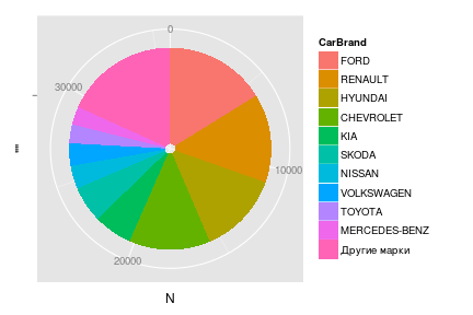
The pie (pie) chart, Pie Chart, is very popular in the business environment, but is subject to valid criticism of data analysis professionals. However, it must be able to "cook."
Suppose you want to display the distribution of the number of taxi licenses, by cars. In order not to overload the chart, we will show only brands with a number of licenses of at least 1000.

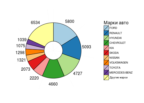
 st <- dt[, list(N = length(RegPlate)), by = CarBrand ] # Summary table st <- st[, CarBrand := reorder(CarBrand, N) ] piedata <- rbind( st[ N >= 1000 ][ order(N, decreasing=T) ], data.table( CarBrand = " ", N = sum( st[N < 1000]$N) ) ) piedata

 ## CarBrand N ## 1: FORD 5800 ## 2: RENAULT 5093 ## 3: HYUNDAI 4727 ## 4: CHEVROLET 4660 ## 5: KIA 2220 ## 6: SKODA 2073 ## 7: NISSAN 1321 ## 8: VOLKSWAGEN 1298 ## 9: TOYOTA 1075 ## 10: MERCEDES-BENZ 1039 ## 11:   6534

To build a graph, I would like to fix just such a sequence of brands. If this is not done, the automatic sorting will display “Other brands” from last place to first.

 piedata <- piedata[, CarBrand := factor(CarBrand, levels = CarBrand, ordered = TRUE)]

To build a chart, use ggplot2.

 pie <- ggplot(piedata, aes( x = "", y = N, fill = CarBrand)) + geom_bar(stat = "identity") + coord_polar(theta = "y") pie

The conclusion is already quite informative. However, I would like to make a number of visual improvements:

remove gray background, borders, rotary axis, signatures and marks;
choose a more distinguishable color scale and circle each “piece of cake”;
next to each sector, put down the number of licenses corresponding to the brand;
give the text a name to the legend.

The code below allows you to do all of the following. To display the labels next to the sectors, we had to add a field with the calculation of the center point of the sector (as found by artelstatistikov.ru ).

 piedata <- piedata[, pos := cumsum(N) - 0.5*N ] pie <- ggplot(piedata, aes( x = "", y = N, fill = CarBrand)) + geom_bar( color = "black", stat = "identity", width = 0.5) + geom_text( aes(label = N, y = pos), x = 1.4, color = "black", size = 5) + scale_fill_brewer(palette = "Paired", name = " ") + coord_polar(theta = "y") + theme_bw() + theme ( panel.border = element_blank() , panel.grid.major = element_blank() , axis.ticks = element_blank() , axis.title.x = element_blank() , axis.title.y = element_blank() , axis.text.x = element_blank() , legend.title = element_text(face="plain", size=16) ) pie

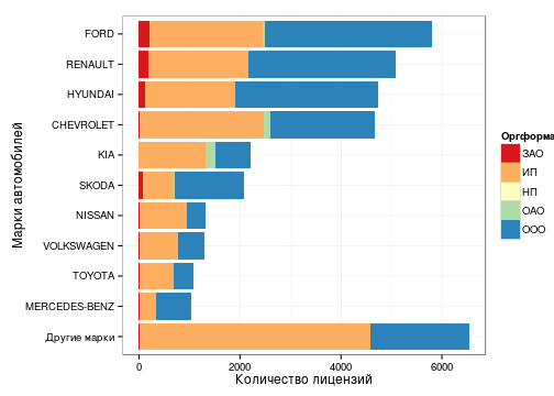
2. Bar graph

A more informative alternative to the circle is the bar chart, Bar Chart. Besides the fact that the lengths of the bars are more convenient to compare than the lengths of the arcs or the areas of the sectors of a circle, the bar chart can additionally display, for example, the distribution of the number of licenses by organizational form.

 st <- dt[, list(N = length(RegPlate)), by = list(OrgType, CarBrand) ] # Summary table cbsort <- st[, list( S = sum(N) ), keyby = CarBrand ] # Order by total number setkey(st, CarBrand) st <- st[cbsort] # Join topcb <- st[ S >= 1000 ][ order(S) ] bottomcb <- st[S < 1000, list(CarBrand = " ", OrgType, N = sum(N)), by = OrgType] bottomcb <- bottomcb[, list(CarBrand, OrgType, N, S = sum(N))] bardata <- rbind( bottomcb, topcb) bardata <- bardata[, CarBrand := factor(CarBrand, levels = unique(CarBrand), ordered=T)] # bar <- ggplot(bardata, aes(x = CarBrand, weight = N, fill = OrgType)) + geom_bar() + coord_flip() + scale_fill_brewer(palette = "Spectral", name = "") + labs(list(y = " ", x = " ")) + theme_bw() bar

3. Heat Map Chart

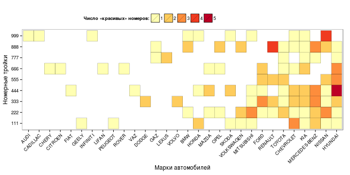
Suppose you want to get an answer to the question: "Owners of what brands of cars (among taxi drivers) are most susceptible to fashion for" beautiful "numbers?". Beautiful in this case, we will consider numbers with the same numbers in triples: 111, 222, etc.
The analysis is carried out on two analytical measurements - car brand and troika. Indicator - the number of cars with a given combination of brand and troika. For visualization of such a data set, a visual analogue of the table is well suited - a heat map diagram. The more popular the triple, the more intense the color encodes the value of the cell.

 ln <- dt[grep( "^[^0-9]([0-9])\\1{2}.+$" , RegPlate), list(CarBrand, LuckyNum = gsub("^[^0-9]([0-9]{3}).+$","\\1", RegPlate))] ln <- ln[, list( N = .N), by = list(CarBrand, LuckyNum) ] ln <- ln[, Luck := sum(N), by = list(CarBrand) ] # Total number of lucky regplates per car brand ln <- ln[, CarBrand := reorder(CarBrand, Luck) ] # heatmap <- ggplot(ln, aes(x = CarBrand, y = LuckyNum)) + geom_tile( aes(fill = as.character(N)), color = "black") + scale_fill_brewer(palette = "YlOrRd", name = " «» :") + labs(list(x = " ", y = " ")) + theme_bw() + theme ( panel.grid.major = element_blank() , axis.text.x = element_text(angle = 45, hjust = 1) , axis.title.y = element_text(vjust = 0.3) , legend.position = "top" , legend.title.align = 1 ) heatmap