Dynamic trees
Before reading the article, I recommend to look at posts about splay-trees ( 1 ) and trees by an implicit key ( 2 , 3 , 4 )
 Dynamic trees (link / cut trees) are poorly lit on the Russian-language Internet. I found only a brief description on algolist. However, this data structure is very interesting. It is located at the junction of two areas: flows and dynamic graphs.
In the first case, dynamic trees allow us to construct efficient algorithms for the problem of finding the maximum flow. Improved algorithms Dynitsa and pre-flow pushes work for and
and  respectively. If you do not know what a stream is and you didn’t have such a thing at lectures, hurry up to replenish your knowledge in Cormen.
')
The second case requires a little introduction. Dynamic graphs are an actively developing modern area of algorithms. Imagine that you have a graph. Changes periodically occur in it: edges appear and disappear, their weights change. Changes need to be quickly processed, and also to be able to efficiently count different metrics, check connectivity, look for diameter. Dynamic trees are a tool that allows you to deftly manipulate with a particular case of graphs, trees.
Before you dive under the cat, try to solve the following problem. Given a weighted graph as a sequence of edges. You can only go through the sequence once. It is required to calculate the minimum spanning tree using memory and
  of time. After reading the article, you will understand how you can easily solve this problem using dynamic trees.
Dynamic trees have many different modifications, sharpened for specific tasks. We will now study the basic version, and then we will finish it on demand.
Imagine that we have a set of trees together vertices. Each tree is suspended by root. We receive the next set of requests.
I want to handle all requests for close to time.
time.
Note that if there were no
Dynamic trees use search trees within themselves. An interesting feature is that with arbitrary balanced trees they process all the above-described requests for depreciation . On splay trees, the same requests are processed depreciated for . Memory used
  .
.
High speed is achieved due to the cunning internal presentation. Divide each tree into a set of paths. Each vertex will lie exactly in one path, and no two paths will intersect. Each path must connect a descendant with an ancestor.

To work with paths, we use search trees with an implicit key. So that there is no confusion in terminology, let's call the trees that we split on the path, represented , and the trees in which we fold these paths, supporting .
The order of the elements in the reference tree is directed so that if you write out all its nodes in order to bypass the left subtree-key-right subtree, then the specified sequence will correspond to the passage of the stored path in the represented tree from the top to the bottom.
Note that the edges that do not participate in the partition always connect the upper vertex of the path with its parent. At each vertex we will store the link. If the vertex is at the top of the path, the link points to its parent. At the root of the tree, the link points to
Here I will only summarize the idea, and all the details, see the post about the Cartesian trees .
Implicit key search trees look like ordinary trees, only the key is not used in them. You can search them th order element. For this, the size of its subtree is recorded in each node. Depending on the size of the left and right subtrees, we choose where to go. It looks something like this:
When balancing the order of the elements in the search trees does not change. Therefore, trees can be considered as smart arrays. you can find -th element, delete it or insert it at the desired position. All operations are feasible for .
If we talk about Cartesian or splay-trees, then we have two additional possibilities: to cut and merge trees. Due to this we can merge and cut the sequence of elements for .
Applied to our problem, search trees using an implicit key allow us to cut one way into two, merge two into one and refer to billing item for .
The key procedure in dynamic trees is

If you have written
Put a link to the parent and run
The first call to
After calling
Let's also find the nearest common ancestor (lowest common ancestor).
The . Let's follow the link to the next support tree and merge it with the previous one. So we will do, until we reach the root of the represented tree.
We will use the auxiliary procedure
Dynamic trees can be expanded to non-root. It is enough to be able to re-hang the trees. Let's look at the following procedure:
The
Adding and deleting edges is trivial.
In the first case,
You can also find the distance between the vertices of one tree.
Operations on the segments provide great opportunities. For example, the maximum flow search algorithms use them to quickly find the bandwidth in the residual network, as well as push the flow along the entire path at once. More details can be found in the book of Tarjan “Data Structures and Network Algorithms”.
Regarding the task in the introduction. The main problem is what to do if a loop appears when adding the next edge. You need to quickly search for the heaviest edge in the path between the given vertices
Technical feature: if the weight of the rib going to the parent is stored in the reference tree at each vertex, then when the root changes, the parents change. The problem can be solved if we store the edge weights to the next and previous vertices along the path. An alternative solution is to create a separate vertex for each edge and only store there the weights.
Let be . The operating time of all the above procedures consists of one or two runs of the
numbers of operations on supporting trees. Operations on reference trees are performed in .
Evaluate the merges and cuts of support trees. This number is expressed by the number of edges that we add to the path under construction. We calculate their total number to get a depreciation estimate.
We assign a weight to each vertex equal to the size of the subtree whose root it is. A rib going from parent to child is called heavy if the weight of the child is strictly more than half the weight of the parent. The remaining ribs are called light.
Statement. The number of light edges on the way from the root to any leaf does not exceed .
.
Each time, going down from the parent to the child along a light edge, the size of the current subtree is reduced at least twice. Since the size of the tree does not exceed , the number of light edges on the way from the root to any leaf does not exceed . 
Based on the previous statement, for all light ribs. Calculate the number of heavy ribs that we add. When adding each heavy rib we will put a coin on it. When the edge no longer lies in the way, we will take this coin. We estimate how many coins we spend.
We can pick up a coin only in two cases: a) time. In the second case, the adjacent selected edge will be light. This can happen no more.
  time. At the end of the work in the tree can be no more
  heavy rib. This means that there are no more total ribs.
  . Thus, the total processing time of all operations
  .
.
In practice, for trees with a small diameter, it is better to use normal
Implementation on python can be found here .
If you read this far, then I congratulate you. I would like to convey a message to two categories of my readers.
The first ones are program students of third and fourth year undergraduate courses. Probably, you didn’t say anything like that at lectures, and you would like to fill in the gaps in the algorithms and many other topics. You have the opportunity to enroll in the magistracy of the Academic University on software development . This is a great chance to replenish your knowledge, put your hand under the supervision of experienced programmers, and for non-residents - to move to Peter. Studying here is not easy, but worth it.
The second are people who wander between Project Euler and Braingames, between Braingames and Topcoder. Are you looking for math problems? Theoretical informatics is great, and there will definitely be a place and a task for you. Look at books about approximate ( 8 , 9 ), exponential ( 10 ), parameterized ( 11 ) algorithms, communication complexity ( 12 ), structural complexity ( 13 ). If it is interesting to you, come to study on theoretical computer science .
Do not miss your opportunity!
Dynamic trees (link / cut trees) are poorly lit on the Russian-language Internet. I found only a brief description on algolist. However, this data structure is very interesting. It is located at the junction of two areas: flows and dynamic graphs.In the first case, dynamic trees allow us to construct efficient algorithms for the problem of finding the maximum flow. Improved algorithms Dynitsa and pre-flow pushes work for
and respectively. If you do not know what a stream is and you didn’t have such a thing at lectures, hurry up to replenish your knowledge in Cormen.')
The second case requires a little introduction. Dynamic graphs are an actively developing modern area of algorithms. Imagine that you have a graph. Changes periodically occur in it: edges appear and disappear, their weights change. Changes need to be quickly processed, and also to be able to efficiently count different metrics, check connectivity, look for diameter. Dynamic trees are a tool that allows you to deftly manipulate with a particular case of graphs, trees.
Before you dive under the cat, try to solve the following problem. Given a weighted graph as a sequence of edges. You can only go through the sequence once. It is required to calculate the minimum spanning tree using
memory and of time. After reading the article, you will understand how you can easily solve this problem using dynamic trees.Formulation of the problem
Dynamic trees have many different modifications, sharpened for specific tasks. We will now study the basic version, and then we will finish it on demand.
Imagine that we have a set of trees together
vertices. Each tree is suspended by root. We receive the next set of requests.make_tree(v)- create a new tree with vertexvlink(u, v)- hang the tree with the root at the vertexuto the vertexv.cut(u, v)- cut the edge (u,v).find_root(v)- find the root of the tree, in which lies the vertexv.depth(v)- find the depth of the vertexv.
I want to handle all requests for close to
time.Note that if there were no
cut and depth queries, the system of disjoint sets ( 5 , 6 , 7 ) could solve this problem.Dynamic trees use search trees within themselves. An interesting feature is that with arbitrary balanced trees they process all the above-described requests for depreciation
. On splay trees, the same requests are processed depreciated for . Memory used .Internal presentation
High speed is achieved due to the cunning internal presentation. Divide each tree into a set of paths. Each vertex will lie exactly in one path, and no two paths will intersect. Each path must connect a descendant with an ancestor.
To work with paths, we use search trees with an implicit key. So that there is no confusion in terminology, let's call the trees that we split on the path, represented , and the trees in which we fold these paths, supporting .
The order of the elements in the reference tree is directed so that if you write out all its nodes in order to bypass the left subtree-key-right subtree, then the specified sequence will correspond to the passage of the stored path in the represented tree from the top to the bottom.
Note that the edges that do not participate in the partition always connect the upper vertex of the path with its parent. At each vertex we will store the link. If the vertex is at the top of the path, the link points to its parent. At the root of the tree, the link points to
None .Implicit Key Search Trees
Here I will only summarize the idea, and all the details, see the post about the Cartesian trees .
Implicit key search trees look like ordinary trees, only the key is not used in them. You can search them
th order element. For this, the size of its subtree is recorded in each node. Depending on the size of the left and right subtrees, we choose where to go. It looks something like this: def find(v, k): if v == None: return None threshold = size(v.left) if k == threshold: return v if k < threshold and v.left != None: return find(v.left, k) if k > threshold and v.right != None: return find(v.right, k - threshold - 1) return None When balancing the order of the elements in the search trees does not change. Therefore, trees can be considered as smart arrays. you can find
-th element, delete it or insert it at the desired position. All operations are feasible for .If we talk about Cartesian or splay-trees, then we have two additional possibilities: to cut and merge trees. Due to this we can merge and cut the sequence of elements for
.Applied to our problem, search trees using an implicit key allow us to cut one way into two, merge two into one and refer to
billing item for .Expose and his friends
The key procedure in dynamic trees is
expose(v) . The procedure rebuilds the paths in the represented tree. We will support the invariant that after the vertex v been requested, it will lie in the same path with the root. Moreover, v will be the final vertex of the path.If you have written
expose , then everything else looks more or less obvious. def link(u, v): u.link = v expose(u) Put a link to the parent and run
expose to support the invariant. def cut(u, v): expose(v) u.link = None expose(u) The first call to
expose we put the vertices u and v in different paths. Feel free to zero the link, and run the second expose to maintain the invariant. def find_root(v): expose(v) return leftest(supportRoot(v)) After calling
expose vertex v and the root will lie in the same reference tree. If the tree is balanced, it is enough to climb to the root, and then go down to the far left node. This will be the root. I conditionally designated the ascent to the root via supportRoot , and the descent to the leftmost element through leftest . In the case of a splay tree, supportRoot is replaced by splay . def depth(v): expose(v) return size(supportRoot(v)) - 1 expose again, again the vertex v and the root in one path. The size of the reference tree is equal to the number of nodes in this path. We rise to the root, find the size of the reference tree. Subtract one to get the number of edges.Let's also find the nearest common ancestor (lowest common ancestor).
def lca(u, v): expose(u) expose(v) return leftest(supportRoot(u)).link Draw on a piece of paper what will happen, and understand that this is really lca. By the way, did you notice that if the vertices lie in different trees, then the procedure will return None? Isn't it very nice of her?The
expose procedure expose boils down to the following: we find the root of the reference tree in which the current node lies; jump to the leftmost element to get to the top of the path. These operations are feasible for . Let's follow the link to the next support tree and merge it with the previous one. So we will do, until we reach the root of the represented tree.We will use the auxiliary procedure
cutout , which cuts off the path on the top of v and puts the necessary links to the children. def expose(v): cutout(v) v = leftest(supportRoot(v)) while v.link != None: cutout(v.link) merge(supportRoot(v.link), (v - v.link), supportRoot(v)) v.link = None v = leftest(supportRoot(v)) return v Non-root trees
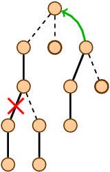
Dynamic trees can be expanded to non-root. It is enough to be able to re-hang the trees. Let's look at the following procedure:
def revert(v): expose(v) reverse(supportRoot(v)) The
revert(v) procedure connects the vertex v with the current root. Note that if the root was a vertex v , then only the order of the elements on the path between v and the root would change. Since the paths are stored in trees by an implicit key, we can implement a turn through delayed operations on segments ( 4 again).Adding and deleting edges is trivial.
def link_edge(u, v): revert(u) link(u, v) def cut_edge(u, v): revert(v) cut(u, v) In the first case,
revert ensures that u is the root of the subtree. In the second, the vertex v will be the parent of u .You can also find the distance between the vertices of one tree.
def dist(u, v): revert(v) return depth(u) Operations on the segments provide great opportunities. For example, the maximum flow search algorithms use them to quickly find the bandwidth in the residual network, as well as push the flow along the entire path at once. More details can be found in the book of Tarjan “Data Structures and Network Algorithms”.
Regarding the task in the introduction. The main problem is what to do if a loop appears when adding the next edge. You need to quickly search for the heaviest edge in the path between the given vertices
u and v . revert from u , expose from v , and we got a reference tree containing this path. Trees using an implicit key allow you to quickly search for the maximum. Therefore, to find the edge is not difficult.Technical feature: if the weight of the rib going to the parent is stored in the reference tree at each vertex, then when the root changes, the parents change. The problem can be solved if we store the edge weights to the next and previous vertices along the path. An alternative solution is to create a separate vertex for each edge and only store there the weights.
Analysis
Let be
. The operating time of all the above procedures consists of one or two runs of the expose procedure and a constantnumbers of operations on supporting trees. Operations on reference trees are performed in
.Evaluate the
expose procedure. Let it consist of merges and cuts of support trees. This number is expressed by the number of edges that we add to the path under construction. We calculate their total number to get a depreciation estimate.We assign a weight to each vertex equal to the size of the subtree whose root it is. A rib going from parent to child is called heavy if the weight of the child is strictly more than half the weight of the parent. The remaining ribs are called light.
Statement. The number of light edges on the way from the root to any leaf does not exceed
.Each time, going down from the parent to the child along a light edge, the size of the current subtree is reduced at least twice. Since the size of the tree does not exceed
, the number of light edges on the way from the root to any leaf does not exceed . Based on the previous statement, for all
expose calls we will add to the path light ribs. Calculate the number of heavy ribs that we add. When adding each heavy rib we will put a coin on it. When the edge no longer lies in the way, we will take this coin. We estimate how many coins we spend.We can pick up a coin only in two cases: a)
expose was caused by the expose and we were cut off, b) a neighboring edge is now on the way. The first case can occur no more time. In the second case, the adjacent selected edge will be light. This can happen no more. time. At the end of the work in the tree can be no more heavy rib. This means that there are no more total ribs. . Thus, the total processing time of all operations .Practical tests
In practice, for trees with a small diameter, it is better to use normal
DFS . Dynamic trees become noticeably efficient when we work with large trees and a large number of link and cut queries. The most high performance is shown on splay-trees. You can find out more in the review of Tarjan, Werneck “Dynamic Trees in Practice” .Implementation on python can be found here .
About life...
If you read this far, then I congratulate you. I would like to convey a message to two categories of my readers.
The first ones are program students of third and fourth year undergraduate courses. Probably, you didn’t say anything like that at lectures, and you would like to fill in the gaps in the algorithms and many other topics. You have the opportunity to enroll in the magistracy of the Academic University on software development . This is a great chance to replenish your knowledge, put your hand under the supervision of experienced programmers, and for non-residents - to move to Peter. Studying here is not easy, but worth it.
The second are people who wander between Project Euler and Braingames, between Braingames and Topcoder. Are you looking for math problems? Theoretical informatics is great, and there will definitely be a place and a task for you. Look at books about approximate ( 8 , 9 ), exponential ( 10 ), parameterized ( 11 ) algorithms, communication complexity ( 12 ), structural complexity ( 13 ). If it is interesting to you, come to study on theoretical computer science .
Do not miss your opportunity!
Literature
Source: https://habr.com/ru/post/216733/
All Articles