How to draw a graph on 1C

Describes the implementation in the 1C query language of the method of locating the vertices of the graph on a plane, based on the use of electromechanical analogy. At the same time, the vertices of the graph are represented by the same electric charges, the arcs are represented by springs. The interaction forces of the vertices in this system translate them from a random initial to the desired final position. The processing of drawing graphs “GraphOgraph”, which implements this approach, also shows the dynamics of the process. The graph can be set with the list of edges manually, choose from several predefined examples or form according to the information base.

1. THEORETICAL PART

The structure of the graph when using electromechanical analogy is determined by two tables: a table of edges and a table of vertices.
The “Edges” edge table contains three columns: the name of one edge of the edge (Name1), the name of the opposite edge of the edge (Name2), and the elastic value of the spring that is used to simulate the edge (Elasticity).
')

Name1	Name2	Elasticity
Vertex1	Vertex2	Elasticity1
...	...	...
VertexA	VertexB	Elasticity AB

The value of elasticity must be greater, the more closely connected the vertices. If the graph represents a social network, the “resilience” can be proportional to the number of messages between the respective members of the network. If the graph represents a transport system, then the elasticity will be the smaller, the greater the distance between the nodes.
The table of peaks contains two columns: the name of the peak (Name) and the value of the electric charge of the peak (Charge).

Name	Charge
Vertex1	Charge1
...	...
VertexA	Charge

The magnitude of the charge can be proportional to the place that the vertex should occupy in the figure, since a more charged vertex will push the neighboring vertices with greater force. For example, when building a graph of links for Infostar participants, you can use a rating as the value of the peak value (charge).

The current state of the system is determined by a state table containing the current coordinates of the vertices and consisting of columns: the name of the vertex (Name), the current horizontal coordinate (X) and the vertical coordinate (Y). The table of vertices and the state table for simplicity can be combined by recording the charge and current coordinates in a single table “Vertices”.

Name	Charge	X	Have
Vertex1	Charge1	X1	U1
...	...	...	...
VertexA	Charge	HA	UA

The dynamics of the described system can be modeled using the Euler method. It allows you to get the coordinates of the vertices after a short period of time based on the current coordinates, knowing the speed and direction (vector) of movement of each vertex.

For our purposes, it is easier to assume that the speed of movement is proportional to the force acting on the top (movement in a viscous medium). To find the force acting on a specific vertex, you need to add up all the forces acting on it from other vertices. The action force from each vertex will consist of the repulsion force determined by Coulomb's law in proportion to the product of the vertex charges divided by the square of the distance between them. And the force of attraction in the case of a connection (edge). The magnitude of the force of attraction is subject to Hooke's law, that is, it is directly proportional to the product of the elasticity of the bond and the distance between the vertices. As a result, a repulsion force will act horizontally at the vertex A with the coordinates A.X and A.U from the vertex B with the coordinates B.X. and B.U.

(A. - B.) / Distance AB * A.Zaryad * B.Zaryad / ((A.H. - B.Kh) * (A.H. - B.Kh) + (A.Y. - B.Y.) * (A.U. - B.U.))

and the vertical repulsive force

(A.U. - B.U.) / Distance AB * A.Zaryad * B.Zaryad / ((A.K. - B.K.) * (A.K. - B.K.) + (A.U. - B.Y.) * (A.U. - B.U.))

Where

Distance AB = SQRT ((A. - B.) * (A. - B.) + (. - B.) * (. - B.))

Elements of the form (A. - B.) / Distance are the projections of the vector of the direction of the force, having a unit length. Such a vector affects the direction, but does not change the magnitude of the force.

If there is an edge between the vertices, the force of attraction will also act. Horizontally, its value will be determined by the formula

((B.H. - A.H.) / Distance AB) * Elasticity AB * Distance AB,

A vertical formula

((B.U. - A.U.) / Distance AB) * Elasticity AB * Distance AB.

Adding two forces and making the necessary reductions, we obtain the formula of horizontal force

(A. - B.) (A.Zaryad * B.Zaryad / DistanceAB / ((A. - B.) * (. - B.) + (. - .) * (A.U. - B.U.)) - Elasticity AB)

and vertical force

(A.U. - B.U.) (A.Zaryad * B.Zaryad / Distance AB / ((A.Kh. - B.Kh.) * (A.K. - B.Kh.) + (A.U. - B.Y.) * (A.U. - B.U.)) - Elasticity AB)

Moving along X and Y can be obtained by multiplying the sum of the forces acting from all the vertices by the step size in time “Step”. Thus, if the current coordinates of the vertices are known, by applying the indicated formulas, the following coordinates can be obtained, and so on, until the system goes into a steady state, where the sum of the forces acting on each vertex is close to zero.

All of the above is implemented by repeating the execution of one fairly simple query:

CHOOSE Ribs. Name1, Ribs. Name2, Ribs. Elasticity
LIPS RIBS & RIBS AS RIBS
;
CHOOSE Ribs. Name1, Ribs. Name2, Ribs. Elasticity
SPACE Dougie
FROM RIB AS RIB
COMBINE ALL
CHOOSE Ribs. Name2, Ribs. Name1, Ribs. Elasticity
FROM RIB AS RIB
INDEX ON RIBS. Name1, RIBs. Name2
;
SELECT Vertices. Name, Vertices. Charge, Vertices. X, Vertices.
SPACE Vertices
FROM & Vertices AS Vertices
;
CHOOSE
A.Name,
MAXIMUM (A. Zaryad) AS Charge,
MAXIMUM (A.X) + & Pitch * SUM ((A.X - B.H) * (A.Zaryad * B.Zaryad / ((A.H - B.H) * (A.H - B.H) + (A.U. — B.U.) * (A.U. — B.U.)) —There is NULL (Dugi.Rugularity, 0))) AS-X,
MAXIMUM (A.U) + & Pitch * SUM ((A.U - B.U) * (A.Zaryad * B.Zaryad / ((A.H - B.Kh) * (A.H - B.Kh) + (A.U. - B.Y.) * (A.U. - B.Y.)) - THERE IS NULL (Dugi.Prugosti, 0))) HOW Y
OF
Vertices like a
INTERNAL CONNECTION Tops AS B
BY A.Name <> B.Name
LEFT JOINT ARC AS AS ARG
BY A.Name = Dugi.Name1
And (B.Name = Arcs. Name2)
LOAD ON
A.Name

The first packet request introduces a table of edges, arcs are formed in the second of the edges, that is, the forces of the edges are directed both from the first to the second vertex and from the second to the first, in the third request the table of vertices is entered, and in the fourth, the necessary calculations. For this, three tables are joined: the table of vertices A and the table of vertices B according to the condition of inequality of the names of the vertices and the table of arcs according to the condition of coincidence of the names of the ends of the arcs with the names of the vertices. Next, grouping is performed by the vertices of table A, during which the superposition of forces is calculated, which is multiplied by the Step and added to the current coordinates.

Attentive readers will notice that in the formulas the “Distance AB” divider is omitted. This is done due to the fact that in the 1C query language there is no function for calculating the square root SQRT. That is, in this query, it is actually considered that the repulsive force is inversely proportional not to the square of the distance between the vertices, but simply to the distance. Thus, the repulsive force is given excessive long-range action. There is nothing terrible in this, since it is not so essential for the task of drawing graphs. However, in the query actually used in processing, this difficulty is overcome. This is done by calculating the square root using the Heron iteration formula.

Distance AB '= (Distance AB + Square Distance AB / Distance AB) / 2,

where the previous value of the distance is taken from the previous iteration of the query, and the initial value is one. Such a solution did not slow down the computation much. This mode is included in the processing of the “Law of Coulomb” tick. Also in the real query, additional optimization was carried out: the reloading of arcs and the indexing of arcs in each iteration are excluded, and the sum of squares of distances for each pair of vertices is considered not four times, as in the original query, but one. If desired, in order to exclude the quadratic dependence of the query execution time on the number of vertices, one can divide the plane into cells (or cells) and consider repulsion only for the vertices of neighboring cells. However, so far this optimization has not been carried out and it is not clear how much this is necessary - it is enough to draw graphs from 100 to 200 speed peaks.

As in other problems of the numerical solution of systems of nonlinear differential equations, it is important to choose the time step. A larger step size leads to an increase in the solution speed, but to certain limits, when the dynamic system loses stability. In all the following examples, with charges and elasticity, 1 step was taken equal to 0.2, except graphs of nomenclature groups and contractors, where the step had to be reduced to 0.05. In general, there is a clear rule - the greater the elasticity, the smaller the step.

2. PRACTICAL PART

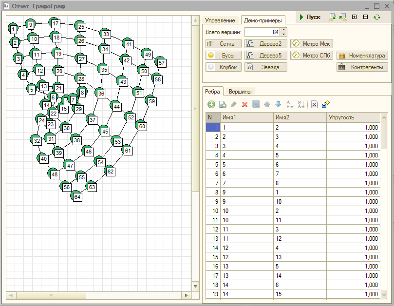
Attached to the article is the “GraphOgraph” (emphasis on the letter “o”). With its help, you can set the structure of the graph and observe the dynamics of its drawing (if the "Show process" checkbox is checked). Processing allows you to change the decision step - it should be positive, but not too large. You can change the moving threshold for stopping - this parameter can be equal to zero, but then you have to interrupt the modeling process manually (Ctrl-Break). You can set the required graph size in millimeters - the graph is automatically scaled, trying to occupy the specified rectangle. You can increase or decrease the graph, as well as (on the vertex tab), rotate it clockwise or counterclockwise, or mirror it (relative to the diagonal). You can set the color of the edges and the color of the vertices (all at the same time - a different color for each vertex and edge is set until it was necessary). In addition, by setting the first edge elasticity, using the “Compare” button, you can make the elasticity of all edges the same as that of the first edge. A similar action is programmed to charge the vertices. Here is what the processing control panel looks like:



The structure of the graph can be set manually by specifying its list of edges. The connected vertices are identified by the names represented by text strings. In a specific application, processing can be specialized so that the vertices are specified by references to the objects of the information base. Then decoding will allow you to open the corresponding objects. The list of vertices when editing edges is formed automatically (charge can be corrected). Dialed parameters and graph structure can be saved as report settings.

If there is no graph whose picture you want to see, you can work with ready-made demo examples. In this case, you can choose the number of vertices of the example graph (by default, 64).

The following are the figures obtained for the hard-wired examples. The dynamics of construction (and it is also very interesting) is better to see by running the processing.

1. Grid (adjacent vertices are connected to cells of a rectangular grid)

2. Necklace (tops are connected in a ring)

3. Clew (all vertices are directly connected)

To get this beautiful picture, it was necessary to zero the elasticity of the ribs in the middle of the ring. Otherwise the view would be completely different:

4. Binary tree

5. 5-ary tree

6. Star (all vertices are connected to one central vertex)

the inherent deficiency of the method is clearly visible here - a straight edge 1–13 does not bypass vertex 5, but crosses it.

7. Metro Moscow

With an increase in the figure, the scheme is well read. The proof is a fragment of the central part with a large increase

8. Metro Peter

Anyone who knows Peter will notice that Vasileostrovskaya and Primorskaya stations are not in their place, but there's nothing you can do - this is a model.

9. Group graph of the Nomenclature reference book (such directory must exist in the configuration where the processing starts)

10. The group graph of the directory "Counterparties" (this directory must also exist in the configuration where the processing starts)

As for the metro schemes, it can be added that when constructing them, I had to go for a certain trick. The fact is that, due to the initial random arrangement of the stations, the long radial branches behind the ring line (for Moscow) are most likely overlapped and then no longer straightened. It would be possible to (a) build a graph by building up stations (how the metro was built), (b) connect the middle stations of the departure branches by a large virtual ring with weak “straightening” connections, (c) fix the end stations or (d) take the district into account when the stations are initially dispersed station. The last method was chosen. It is also worth noting that the number (187 with regard to the like) stations of the Moscow metro is already close to the limit of the method capabilities. In the status bar when the method is running, the number of frames per second that processing time manages is noted. For example, the metro processing (file base, laptop, process display disabled and Coulomb's law) showed approximately 2.4 fps. The structure of the metro is recorded in the processing layouts, if you wish, you can add an image of any other metro.

All other figures are built almost instantly or rather quickly and fully automatically according to information only about the structure of graphs. Only scaling and rotation was used. The relatively small number of vertices depicted in the examples is explained not by the limited capabilities of the method, but by the desire to make the drawings smaller.

It seems that these examples should be sufficient to prove the efficiency and practical applicability of the method. But the representation of relations in the form of graphs is so universal that, without a doubt, there are still many other illustrative examples. In particular, it was possible to build another family tree, a structure of comments for the selected article on Infostarte, user connections “1C: Document Management” and so on and so forth. By adding a few lines of code, you can draw arrows on arcs and, thus, draw oriented graphs.

It is possible to suggest other ways of “configuring” this “typical” model for a specific task, in addition to vertices-objects, multi-colored vertices, multi-colored arcs and arrows on them. For example, it is extremely easy to add a third dimension and solve the problem of placing vertices in space. You can fix some vertices, each time zeroing the calculated movement. After that, you can add a “flow” so that the peaks “relate” to the desired direction. Well, either to introduce the force of pushing away vertices and from arcs too, in order to correct the inherent disadvantage of the considered algorithm - the intersection of arcs of “alien” vertices.

FINDINGS

As a result, according to the results of testing the processing on the listed examples, we can draw the following conclusions: the method works ideally in the case of relatively weak graphs of a symmetric and regular structure. In the case of the other extreme - a complicated entangled structure of the graph, sometimes (but not always!) It may be necessary to manually correct some parameters (step, charge, repulsion law, elasticity, current coordinates) or even the choice of a fundamentally different algorithm. There are limitations (in theory - surmountable) and the size of the graph. But, on the other hand, unlike other algorithms, the implementation of this method is feasible on a pure 1C without using any external components by a simple query of 14 lines (in the main part).

Well, in general, the considered approach once again shows the flexibility of the query language and the extent to which scientific disciplines are interconnected. In solving this particular practical problem of automation, knowledge was required from several different areas of mathematics and physics. Even the Pythagorean theorem was useful. In general, knowledge is power!

File processing

(C) ildarovich