Animated graphics in R (and a little about bifurcation, chaos and attractors)

Once I needed animated graphics for the presentation. With the graphs, in fact, there were no problems, and for their animation I had to use another animation package that can be installed from CRAN.

 install.packages("animation") library(animation) 

It should be noted that animation uses the ImageMagick software package during image processing, so it is advisable to install it in advance. Under Windows, I did not test the performance of this solution.
To create animated graphics, we, in general, need only one function of this type:

 saveGIF({ # - ,    }, movie.name=..., interval=..., ani.width=..., ani.height=...) 

It so happened that at that time I was taking a very cognitive course on Introduction to Dynamic Systems and Chaos , and I was wondering how they move from relatively simple mathematical objects to very fancy images. Take at least a logistic mapping of this type:

This iterative function can be interpreted as the dependence of the population size on its size in the previous period of time and on the parameter r , which is usually called the reproduction rate. Actually, the function itself is rather dull and has a very trite schedule. Interesting things manifest themselves if we consider its bifurcation diagram : by changing the parameter r , we can observe the “dynamics” of the fixed points of the equation . We write the logistic mapping in R as such a function:

 logistic.map <- function(r, x0, n, m){ x <- rep(x0, n) for(i in 1:(n-1)) { x[i+1] <- r * x[i] * (1 - x[i]) } return(x[(nm):n]) } 

Let us set some interesting points and initial parameters for the display and construct a bifurcation diagram, zooming along the way:

As a result, we get something like this:

You can see that the number of fixed points of the equation is doubled, thus forming a cascade of bifurcations and manifesting a fractal structure. Here it is still appropriate to recall such a phenomenon as universality. Consider two equations:


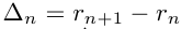
The first equation determines the distance from one point of bifurcation to the next in units of r . The second shows how much branch n is longer than branch n + 1. So, it turns out that

The number 4.669201 ... is called the universal Feigenbaum constant , which just characterizes the speed of transition of dynamical systems from order to deterministic chaos.

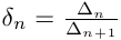
Another interesting and equally famous object is the Lorenz attractor . On Habré, he even has a separate article . To describe the movement of airflows, Edward Lorenz used a system of three ordinary differential equations, now known as the Lorentz equations:

We will not get lost and solve this system numerically - by the Euler method :

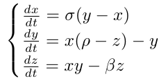
 lorenz.solution <- function(sigma=10, r=28, beta=8/3, x=0.01, y=0.01, z=0.01, dt=0.001, n=30000){ sol <- array(0, dim=c(n,3)) t <- 0 for(i in 1:n){ x0 <- x; y0 <- y; z0 <- z x <- x0 + (y0 - x0) * sigma * dt y <- y0 + ((r - z0) * x0 - y0) * dt z <- z0 + (x0 * y0 - beta * z0) * dt t <- t + dt sol[i,] <- c(x, y, z) } return(sol) } 

The system solution for the default parameters looks like this:

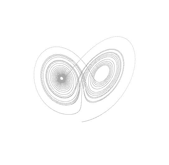
By changing the parameter r, one can get a series of images, which show how the system evolves from the initial conditions and the fixed point to the strange attractor itself .

 library(scatterplot3d) saveGIF({ for (r in 2:34){ sol <- lorenz.solution(r=r) s3d<-scatterplot3d(sol[,1], sol[,2], sol[,3], color="gray66", angle=15, box=F, grid=F, axis=F, pch=".", main=paste0("Lorenz Attractor with rho=", r)) } }, movie.name = "lorenz.gif", interval=.3, ani.width=500, ani.height=500) 

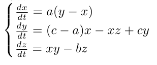
Attractor Lorenz is not the only one of its kind. For example, the Chen attractor is described as:


The orbits along which the motion occurs are “tightened” to the attractor; this movement is chaotic and sensitive to the initial conditions, at the same time it is stable globally. David Feldman, who teaches the course “Introduction to Dynamic Systems and Chaos”, says that although it is difficult to predict the state of a particular point in chaotic systems, the statistical parameters of such systems are quite accurately defined. Thus, it can be argued about the statistical predictability of the system. For example, the weather at a particular minute, strictly speaking, is unpredictable, but the climate has quite certain parameters. And there is no contradiction in this.