Random Forest model for classification, implementation on c #

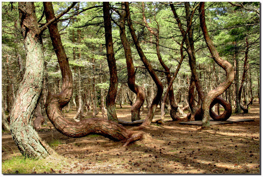Good day, reader. Random Forest today is one of the most popular and extremely effective methods for solving machine learning problems, such as classification and regression. In terms of efficiency, it competes with support vector machines, neural networks and boosting, although of course it is not without its drawbacks. In appearance, the learning algorithm is extremely simple (in comparison, let's say with the support vector machine learning algorithm, to whom there is little thrill in life, I strongly advise you to do this at your leisure). We will try to understand the basic ideas of Random Forest (binary decision tree, bootstrap aggregation or bagging, the method of random subspaces and decorrelation) in an accessible form and understand why all this works together. The model with respect to its competitors is still quite young: it all started with a 1997 article in which the authors proposed a method for constructing a single decision tree using the method of random subspaces of signs when creating new tree nodes; Then there was a series of articles, which ended with the publication of a canonical version of the algorithm in 2001 , in which an ensemble of decision trees was built based on bootstrap aggregation, or bugging. At the end, a simple, not at all smart, but extremely visual way of implementing this model in c # will be given, as well as a series of tests. By the way, in the photo on the right you can see a real random forest that grows here in the Kaliningrad region on the Curonian Spit .

Binary decision tree

It should start with a tree, as with the main structural element of the forest, but in the context of the model under study. The presentation will be based on the assumption that the reader understands what a tree is, as a data structure . The tree will be built approximately according to the CART (Classification and Regression Tree) algorithm , which builds binary decision trees. By the way, here on Habré there is a good article on building such trees based on entropy minimization , in our version this will be a special case. So imagine the feature space, let's say two-dimensional, that would be easier to visualize, in which a set of objects of two classes is given.

We introduce a series of notation. Denote the set of features as follows:

For each feature, you can select a set of its values, based either on the training set, or using other a priori information about the task, we denote as follows a finite set of characteristic values:

It is also necessary to introduce the so-called measure of heterogeneity of a set relative to its labels. Imagine that a subset of the training set consists of 5 red and 10 blue objects, then we can say that in this subset the probability of pulling out the red object will be 1/3 , and the blue 2/3 . Let us denote the probability of the k-th class as follows in some subset of the training set:

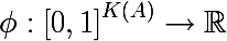
Thus, we have defined an empirical discrete probability distribution of labels in a subset of observations. A measure of the heterogeneity of this subset is called a function of the following form, where K (A) is the total number of labels of the subset A :

The measure of heterogeneity is set in such a way that the value of the function increases as far as possible with increasing set variance , reaching its maximum when the set consists of the same number of various labels, and the minimum if the set consists only of the labels of one class (once again I advise you to look at entropy example with pictures ).
')
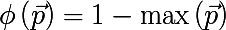
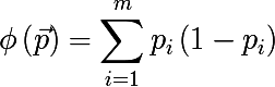
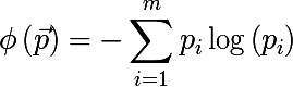
Let's take a look at some examples of measures of heterogeneity (the vector p consists of m probabilities of the marks found in a certain subset A of the training set):

Most commonly occurring class:
Gini index :
Cross-entropy :

The algorithm for constructing a binary decision tree works according to the greedy algorithm scheme: at each iteration for the input subset of the training set, such a partition of space is constructed by a hyperplane (orthogonal to one of their coordinate axes) that would minimize the average measure of heterogeneity of the two subsets obtained. This procedure is performed recursively for each resulting subset until the stopping criteria are reached. Let us write this more formally; for the input set A, we find a pair of < attribute , characteristic value >, that the measure of heterogeneity will be minimal:

Where

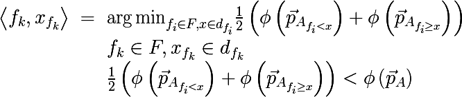
- the probability vector obtained by the above procedure from a subset of the set A , consisting of those elements for which the condition f <x is satisfied. Also, do not forget that the average cost of a partition should not exceed the cost of the original set. Let's now go back to the original picture and look at what is really happening, divide the original set of data as described above:

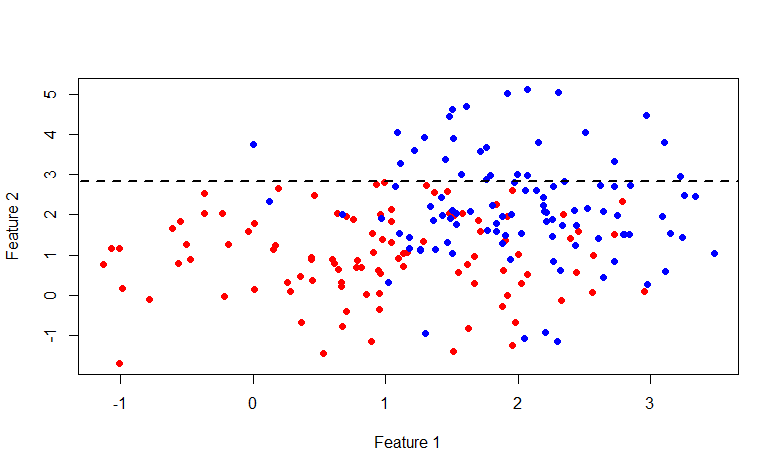
As you can see, the set above the line y = 2.840789 consists entirely of blue marks, so it has washed away to break further only the second set.

This time the line is x = 2.976719 . In general, it is interesting to indulge with this picture, here is the code for R:

Visualization code

rm(list=ls()) library(mvtnorm) labCount <- 100 lab1 <- rmvnorm(n=labCount, mean=c(1,1), sigma=diag(c(1, 1))) lab0 <- rmvnorm(n=labCount, mean=c(2,2), sigma=diag(c(0.5, 2))) df <- data.frame(x=append(lab1[, 1], lab0[, 1]), y=append(lab1[, 2], lab0[, 2]), lab=append(rep(1, labCount), rep(0, labCount))) plot(df$x, df$y, col=append(rep("red", labCount), rep("blue", labCount)), pch=19, xlab="Feature 1", ylab="Feature 2") giniIdx <- function(data) { p1 <- sum(data$lab == 1)/length(data$lab) p0 <- sum(data$lab == 0)/length(data$lab) return(p0*(1 - p0) + p1*(1 - p1)) } p.norm <- giniIdx getSeparator <- function(data) { idx <- NA idx.val <- NA cost <- p.norm(data) for(i in 1:(dim(data)[2] - 1)) { for(i.val in unique(data[, i])) { #print(paste("i = ", i, "; v = ", i.val, sep="")) cost.tmp <- 0.5*(p.norm(data[data[, i] < i.val, ]) + p.norm(data[data[, i] >= i.val, ])) if(is.nan(cost.tmp)) { next } if(cost.tmp < cost) { cost <- cost.tmp idx <- i idx.val <- i.val } } } return(c(idx, idx.val)) } s1 <- getSeparator(df) lines(c(-100, 100), c(s1[2], s1[2]), lty=2, lwd=2, type="l")

We list the possible stopping criteria: the maximum depth of the node has been reached; the probability of the dominant class in the partition exceeds some threshold (I use 0.95); the number of elements in the subset is less than a certain threshold. As a result, we get a partition of the whole set into (hyper) rectangles, and each such subset of the learning set will be associated with one leaf of the tree, and all internal nodes are one of the partitioning conditions; or in other words some predicate. At the current node, the left descendant is associated with those elements of the set for which the predicate is true, and the right one, respectively, with the topic for which the predicate returns false. It looks something like this:

So we got a tree, how to make a decision on it? It will not be difficult for us to determine to which of the subsets of the training set any input image belongs, in the opinion of a particular decision tree. Then we just have to choose the dominant class in this subset and return it to the client, or return the probability distribution of labels in this subset.

By the way at the expense of the regression task. The described tree construction method easily changes from the classification problem to the regression problem. For this, it is necessary to replace the measure of heterogeneity with a certain measure of forecasting error, for example, the standard deviation. And when deciding, instead of the dominant class, the average value of the target variable is used.

It seems with the trees all decided. We will not dwell on the pros and cons of this method, there is a good list in Wikipedia . But in the end I want to add an illustration from the book An Introduction to Statistical Learning about the difference of linear models and trees.

This illustration shows the difference between a linear model and a binary decision tree, as you can see in the case of linear separability, in general, the tree will show a less accurate result than a simple linear classifier.

Bootstrap aggregating or bagging

Let's move on to the next ideological component of random forest. So the name BAG ging, formed from B ootstrap AG gregating. In statistics, bootstrap is understood as a method for estimating the standard error of the statistics of a sample probability distribution, and a method for sampling samples from a data set based on the Monte Carlo method .

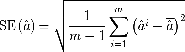
Bootstrap sampling is quite simple in its idea, and is used when we are unable to obtain a large number of samples from the actual distribution, and this is almost always the case. Suppose we want to get m sets of observations of size n , but we have only one set of n observations at our disposal. Then we generate m sets by equiprobable selection of n elements from the original set with the return of the selected element ( sampling with repetition or return ). For large values of n , the number of unique elements obtained by bootstrap sampling sets will be (1 - 1 / e) ≈ 63.2% of the total number of unique observations of the original set. Denote by D ⁱ - the i -th set obtained by bootstrapping by sampling, we estimate on it some parameter a ⁱ , and repeat this procedure m times. The standard error of the parameter estimation bootstrap is written as follows:

So, the statistical bootstrap allows us to estimate the error in estimating a certain distribution parameter. But this is a distraction from the topic, we are also interested in the bootstrap sampling method.

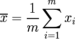
Now consider a set of m independent randomly selected elements x from one probability distribution, with some expectation and variance σ ² . Then the sample average will be equal to:

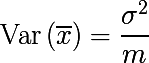
The sample mean is not a distribution parameter, unlike the expectation and variance, but a function of random variables, i.e. is also a random variable, from a certain probability distribution of sample means. And it, in turn, has the variance parameter, which is expressed as follows:

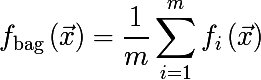
It turns out that averaging the set of values of a random variable reduces variability . This is the basis for the idea of aggregating bootstrap samples. Generate m bootstrap samples of size n from the training set D (also of size n ):

At each bootstrap sample, we train model f and introduce the following function, this approach is called bootstrap aggregating or bagging:

Bagging can be illustrated by the following wikipedia chart , where the bag model is represented by a red line and is the averaging of many other models.

Decorrelation

I think it is already clear how to get a simple forest: we will generate some amount of bootstrap samples and train a decision tree on each of them. But there is a small problem, almost all trees will be more or less the same structure. Let's do an experiment, take a set with two classes and 32 features , build 1000 decision trees on bootstrap samples, and look at the variability of the predicate of the root node.

We see that of 1000 trees, the 22nd feature (obviously, the value of the feature is the same) occurs in 526 trees, and almost all the child nodes are the same. In other words, the trees are correlated relative to each other. It turns out that it makes no sense to build 1000 trees, if only a few, but most often one or two is enough. And now let's try to use in the construction of a tree, when dividing each node, only some small random set of features from the set of all features, say 7 random ones from 32.

As you can see, the distribution has significantly changed in the direction of a greater variety of trees (by the way, not only in the root node, but also in the subsidiaries), which was the goal of such a trick. Now 22 signs are found only in 158 cases. The choice of " 7 random of 32 signs" is justified by empirical observation (I never found the author of this observation), and in classification problems this is usually the square root of the total number of signs. In other words, trees have become less correlated , and the process is called decorrelation .

Such a method is generally called the Random subspace method and is used not only for decision trees, but also for other models, such as neural networks.

In general, something like this would look like a regular flat forest, and decorrelated.

Code

Let's turn to implementation. Once again I want to remind you that the example I have cited is not a quick implementation of random forest, but is of an educational nature only, designed to help understand the basic ideas of the model. For example, here you will find an example of a suitable and quick implementation , but unfortunately less understandable.

Comments I will insert where necessary right in the code, so as not to break the classes into pieces.

Plain tree

 //   ,            public class TreeNode<T> { public TreeNode() { Childs = new LinkedList<TreeNode<T>>(); } public TreeNode(T data) { Data = data; Childs = new LinkedList<TreeNode<T>>(); } public TreeNode<T> Parent { get; set; } public LinkedList<TreeNode<T>> Childs { get; set; } public T Data { get; set; } public virtual bool AddChild(T data) { TreeNode<T> node = new TreeNode<T>() {Data = data}; node.Parent = this; Childs.AddLast(node); return true; } public virtual bool AddChild(TreeNode<T> node) { node.Parent = this; Childs.AddLast(node); return true; } public bool IsLeaf { get { return Childs.Count == 0; } } public int Depth { get { int d = 0; TreeNode<T> node = this; while (node.Parent != null) { d++; node = node.Parent; } return d; } } }

The unit of observation in my case is represented by the following class.

Observation

 public class DataItem<T> { private T[] _input = null; private T[] _output = null; public DataItem() { } public DataItem(T[] input, T[] output) { _input = input; _output = output; } public T[] Input { get { return _input; } set { _input = value; } } public T[] Output { get { return _output; } set { _output = value; } } }

For each node of the tree, it is necessary to store information about the predicate, which is used to make a classification decision.

Tree node data

 public class ClassificationTreeNodeData { //   <id ,  >,         //    p      internal IDictionary<double, double> Probabilities { get; set; } //   ,   ,         //         internal double Cost { get; set; } //       ,   , //    ,            -) internal Predicate<double[]> Predicate { get; set; } //     ,       internal IList<DataItem<double>> DataSet { get; set; } //  ,     internal string Name { get; set; } //        internal int FeatureIndex { get; set; } //       internal double FeatureValue { get; set; } //            ,    [OnSerializing] private void OnSerializing(StreamingContext context) { Predicate = null; } [OnDeserialized] [OnSerialized] private void OnDeserialized(StreamingContext context) { Predicate = v => v[FeatureIndex] < FeatureValue; } }

Consider a binary decision tree class.

Binary deciding tree

 public class ClassificationBinaryTree { private TreeNode<ClassificationTreeNodeData> _rootNode = null; private INorm<double> _norm = null; //    private int _minLeafDataCount = 1; //         private int[] _trainingFeaturesSubset = null; //         private int _randomSubsetSize = 0; //   ,      private Random _random = null; private double _maxProbability = 0; //   ,        private int _maxDepth = Int32.MaxValue; //    private bool _showLog = false; private int _featuresCount = 0; public ClassificationBinaryTree(INorm<double> norm, int minLeafDataCount, int[] trainingFeaturesSubset = null, int randomSubsetSize = 0, double maxProbability = 0.95, int maxDepth = Int32.MaxValue, bool showLog = false) { _norm = norm; _minLeafDataCount = minLeafDataCount; _trainingFeaturesSubset = trainingFeaturesSubset; _randomSubsetSize = randomSubsetSize; _maxProbability = maxProbability; _maxDepth = maxDepth; _showLog = showLog; } public TreeNode<ClassificationTreeNodeData> RootNode { get { return _rootNode; } } //   public void Train(IList<DataItem<double>> data) { _featuresCount = data.First().Input.Length; if (_randomSubsetSize > 0) { _random = new Random(Helper.GetSeed()); } IDictionary<double, double> rootProbs = ComputeLabelsProbabilities(data); _rootNode = new TreeNode<ClassificationTreeNodeData>(new ClassificationTreeNodeData() { DataSet = data, Probabilities = rootProbs, Cost = _norm.Calculate(rootProbs.Select(x => x.Value).ToArray()) }); //    Queue<TreeNode<ClassificationTreeNodeData>> queue = new Queue<TreeNode<ClassificationTreeNodeData>>(); queue.Enqueue(_rootNode); while (queue.Count > 0) { if (_showLog) { Logger.Instance.Log("Tree training: queue size is " + queue.Count); } TreeNode<ClassificationTreeNodeData> node = queue.Dequeue(); int sourceCount = node.Data.DataSet.Count; //   TrainNode(node, node.Data.DataSet, _trainingFeaturesSubset, _randomSubsetSize); if (_showLog && node.Childs.Count() > 0) { Logger.Instance.Log("Tree training: source " + sourceCount + " is splitted into " + node.Childs.First().Data.DataSet.Count + " and " + node.Childs.Last().Data.DataSet.Count); } //       foreach (TreeNode<ClassificationTreeNodeData> child in node.Childs) { if (child.Data.Probabilities.Count == 1 || child.Data.DataSet.Count <= _minLeafDataCount || child.Data.Probabilities.First().Value > _maxProbability || child.Depth >= _maxDepth) { child.Data.DataSet = null; continue; } queue.Enqueue(child); } } } //   private void TrainNode(TreeNode<ClassificationTreeNodeData> node, IList<DataItem<double>> data, int[] featuresSubset, int randomSubsetSize) { // argmin  double minCost = node.Data.Cost; int idx = -1; double threshold = 0; IDictionary<double, double> minLeftProbs = null; IDictionary<double, double> minRightProbs = null; IList<DataItem<double>> minLeft = null; IList<DataItem<double>> minRight = null; double minLeftCost = 0; double minRightCost = 0; //     ,   if (randomSubsetSize > 0) { featuresSubset = new int[randomSubsetSize]; IList<int> candidates = new List<int>(); for (int i = 0; i < _featuresCount; i++) { candidates.Add(i); } for (int i = 0; i < randomSubsetSize; i++) { int idxRandom = _random.Next(0, candidates.Count); featuresSubset[i] = candidates[idxRandom]; candidates.RemoveAt(idxRandom); } } else if (featuresSubset == null) { featuresSubset = new int[data.First().Input.Length]; for (int i = 0; i < data.First().Input.Length; i++) { featuresSubset[i] = i; } } //     foreach (int i in featuresSubset) { IList<double> domain = data.Select(x => x.Input[i]).Distinct().ToList(); //        foreach (double t in domain) { IList<DataItem<double>> left = new List<DataItem<double>>(); //      IList<DataItem<double>> right = new List<DataItem<double>>(); //    IDictionary<double, double> leftProbs = new Dictionary<double, double>(); //      IDictionary<double, double> rightProbs = new Dictionary<double, double>(); foreach (DataItem<double> di in data) { if (di.Input[i] < t) { left.Add(di); if (!leftProbs.ContainsKey(di.Output[0])) { leftProbs.Add(di.Output[0], 0); } leftProbs[di.Output[0]]++; } else { right.Add(di); if (!rightProbs.ContainsKey(di.Output[0])) { rightProbs.Add(di.Output[0], 0); } rightProbs[di.Output[0]]++; } } if (right.Count == 0 || left.Count == 0) { continue; } //   leftProbs = leftProbs.ToDictionary(x => x.Key, x => x.Value/left.Count); rightProbs = rightProbs.ToDictionary(x => x.Key, x => x.Value/right.Count); double leftCost = _norm.Calculate(leftProbs.Select(x => x.Value).ToArray()); //    double rightCost = _norm.Calculate(rightProbs.Select(x => x.Value).ToArray()); double avgCost = (leftCost + rightCost)/2; //    if (avgCost < minCost) { minCost = avgCost; idx = i; threshold = t; minLeftProbs = leftProbs; minRightProbs = rightProbs; minLeft = left; minRight = right; minLeftCost = leftCost; minRightCost = rightCost; } } } //         node.Data.DataSet = null; if (idx != -1) { //node should be splitted node.Data.Predicate = v => v[idx] < threshold; //        node.Data.Name = "x[" + idx + "] < " + threshold; node.Data.Probabilities = null; node.Data.FeatureIndex = idx; node.Data.FeatureValue = threshold; node.AddChild(new ClassificationTreeNodeData() { Probabilities = minLeftProbs.OrderByDescending(x => x.Value).ToDictionary(x => x.Key, x => x.Value), DataSet = minLeft, Cost = minLeftCost }); node.AddChild(new ClassificationTreeNodeData() { Probabilities = minRightProbs.OrderByDescending(x => x.Value).ToDictionary(x => x.Key, x => x.Value), DataSet = minRight, Cost = minRightCost }); } } //     ,     private IDictionary<double, double> ComputeLabelsProbabilities(IList<DataItem<double>> data) { IDictionary<double, double> p = new Dictionary<double, double>(); double denominator = data.Count; foreach (double label in data.Select(x => x.Output[0]).Distinct()) { p.Add(label, data.Where(x => x.Output[0] == label).Count() / denominator); } return p; } //    public IDictionary<double, double> Classify(double[] v) { TreeNode<ClassificationTreeNodeData> node = _rootNode; while (!node.IsLeaf) { node = node.Data.Predicate(v) ? node.Childs.First() : node.Childs.Last(); } return node.Data.Probabilities; } //     GraphVis http://www.graphviz.org/ public void WriteDotFile(StreamWriter sw, bool separateTerminalNode = false) { sw.WriteLine("digraph G{"); sw.WriteLine("graph [ordering=\"out\"];"); Queue<TreeNode<ClassificationTreeNodeData>> q = new Queue<TreeNode<ClassificationTreeNodeData>>(); q.Enqueue(_rootNode); int terminalCount = 0; ISet<string> styles = new HashSet<string>(); while (q.Count > 0) { TreeNode<ClassificationTreeNodeData> node = q.Dequeue(); foreach (TreeNode<ClassificationTreeNodeData> child in node.Childs) { string childName = child.Data.Name; if (String.IsNullOrEmpty(childName)) { if (separateTerminalNode) { childName = "TNode #" + terminalCount + "; Class: " + child.Data.Probabilities.First().Key; } else { childName = "Class: " + child.Data.Probabilities.First().Key; } styles.Add("\"" + childName + "\" [" + "color=red, style=filled" + "];"); terminalCount++; } sw.WriteLine("\"" + node.Data.Name + "\" -> " + "\"" + childName + "\";"); q.Enqueue(child); } } foreach (string style in styles) { sw.WriteLine(style); } sw.WriteLine("}"); } }

Let us dwell on the norm used in the class of the decision tree.

Interface norm

 public interface INorm<T> { double Calculate(T[] v); }

Gini Index

 internal class GiniIndex : INorm<double> { #region INorm<double> Members public double Calculate(double[] v) { return v.Sum(p => p*(1 - p)); } #endregion }

Cross entropy

 internal class MetricsBasedNorm<T> : INorm<T> { private IMetrics<T> _m = null; internal MetricsBasedNorm(IMetrics<T> m) { _m = m; } #region INorm<T> Members public double Calculate(T[] v) { return _m.Calculate(v, v); } #endregion } public interface IMetrics<T> { /// <summary> /// Calculate value of metrics /// </summary> double Calculate(T[] v1, T[] v2); /// <summary> /// Get centroid/clusteroid of data /// </summary> T[] GetCentroid(IList<T[]> data); /// <summary> /// Calculate value of partial derivative by v2[v2Index] /// </summary> T CalculatePartialDerivaitveByV2Index(T[] v1, T[] v2, int v2Index); } internal class CrossEntropy : MetricsBase<double> { internal CrossEntropy() { } /// <summary> /// \sum_i v1_i * ln(v2_i) /// </summary> public override double Calculate(double[] v1, double[] v2) { if (v1.Length != v2.Length) { throw new ArgumentException("Length of v1 and v2 should be equal"); } if (v1.Length == 0 || v2.Length == 0) { throw new ArgumentException("Vector dimension can't be 0"); } double d = 0; for (int i = 0; i < v1.Length; i++) { d += v1[i]*Math.Log(v2[i] + Double.Epsilon); } return -d; } public override double CalculatePartialDerivaitveByV2Index(double[] v1, double[] v2, int v2Index) { return v2[v2Index] - v1[v2Index]; } }

Well, it remains to consider only the class random forest.

Random forest

 public class ClassificationRandomForest { //     ,   private INorm<double> _norm = null; private int _minLeafDataCount = 1; private int[] _trainingFeaturesSubset = null; private int _randomSubsetSize = 0; //zero if all features needed private double _maxProbability = 0; private int _maxDepth = Int32.MaxValue; private bool _showLog = false; private int _forestSize = 0; //   private ConcurrentBag<ClassificationBinaryTree> _trees = null; public ClassificationRandomForest(INorm<double> norm, int forestSize, int minLeafDataCount, int[] trainingFeaturesSubset = null, int randomSubsetSize = 0, double maxProbability = 0.95, int maxDepth = Int32.MaxValue, bool showLog = false) { _norm = norm; _minLeafDataCount = minLeafDataCount; _trainingFeaturesSubset = trainingFeaturesSubset; _randomSubsetSize = randomSubsetSize; _maxProbability = maxProbability; _maxDepth = maxDepth; _forestSize = forestSize; _showLog = showLog; } public void Train(IList<DataItem<double>> data) { if (_showLog) { Logger.Instance.Log("Training is started"); } //     ,       _trees = new ConcurrentBag<ClassificationBinaryTree>(); Parallel.For(0, _forestSize, i => { ClassificationBinaryTree ct = new ClassificationBinaryTree( _norm, _minLeafDataCount, _trainingFeaturesSubset, _randomSubsetSize, _maxProbability, _maxDepth, false ); ct.Train(BasicStatFunctions.Sample(data, data.Count, true)); _trees.Add(ct); if (_showLog) { Logger.Instance.Log("Training of tree #" + _trees.Count + " is completed!"); } }); } // ,      bagging public IDictionary<double, double> Classify(double[] v) { IDictionary<double, double> p = new Dictionary<double, double>(); foreach (ClassificationBinaryTree ct in _trees) { IDictionary<double, double> tr = ct.Classify(v); double winClass = tr.First().Key; if (!p.ContainsKey(winClass)) { p.Add(winClass, 0); } p[winClass]++; } double denominator = p.Sum(x => x.Value); return p.ToDictionary(x => x.Key, x => x.Value/denominator) .OrderByDescending(x => x.Value) .ToDictionary(x => x.Key, x => x.Value); } public IList<ClassificationBinaryTree> Forest { get { return _trees.ToList(); } } }

Conclusion and links

If you looked at the code, you might notice that there is a function in the tree for writing the structure and conditions in the dot format, which is rendered by the GraphVis program . If you run a random forest with the following parameters on the above set :

 ClassificationRandomForest crf = new ClassificationRandomForest( NormCreator.CreateByMetrics(MetricsCreator.CrossEntropy()), 10, 1, null, Convert.ToInt32(Math.Round(Math.Sqrt(ds.TrainSet.First().Input.Length))), 0.95, 1000, true ); crf.Train(ds.TrainSet);

Then the following code will help us visualize this forest:

 foreach (ClassificationBinaryTree tree in crf.Forest) { using (StreamWriter sw = new StreamWriter(@"e:\Neuroximator\NetworkTrainingOCR\TreeTestData\Forest\" + (new DirectoryInfo(@"e:\Neuroximator\NetworkTrainingOCR\TreeTestData\Forest\")).GetFiles().Count() + ".dot")) { tree.WriteDotFile(sw); sw.Close(); } }