Break me down completely (ZeroNightsCrackme, Part 2)
And hello again! Last time, I uncovered the ZeroNightsCrackMe solution. All those who managed to solve it in time could receive an invitation to a tour to one of the offices of Kaspersky Lab, as well as a gift, in the form of a license key for three devices. But, among other things, Kaspersky reported that the crack was lightened, i.e. there is a more complicated version of it and it will be sent out to those who wish to see it (but without gifts, for their own pleasure, so to speak). Of course, I could not deny myself not to twist this version, so I confirmed my desire to participate.
On February 17, a letter arrived with a new quack. It is about his decision (and not only) that I will tell in this article.
Crack options are the same:
Instruments:
Let's get down to solving ...
')
As usual, we run the test subject and perform a surface analysis. The reaction is similar to past quacks.

Fig. one
Knowing the principle of past quack work, let's start searching for key points and find:
After that, we will compare all key points with the previous version and find differences.
First we find the function of processing the entered data. This is done quite simply. Click the right mouse button in the disassembler window and select “Search for => All referenced strings” :

Fig. 2
Next, click on the line "Good work, Serial is valid !!!" and get here:
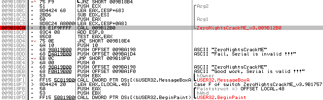
Fig. 3
The above will be the desired function (in my case it is CALL 0x9b12b0 ). It is passed three parameters. In Arg2 , Arg1 , the size of the serial code and the pointer to the serial code are transmitted, respectively, and in the ECX register, the pointer is sent to the email.
Go inside the function and turn to the bottom, there is an algorithm for checking the validation table (identical to the old version):

Fig. four
We set a breakpoint at the beginning of the algorithm and run cracks for execution (of course, first enter any data and click the Check button).

Fig. 5. Enter the test data
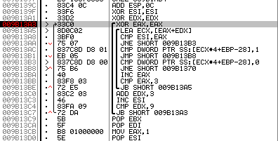
Fig. 6. Stop at the validation table
Now we define the address of the table itself. You can do this by going to the line “CMP DWORD PTR SS: [ECX * 4 + EBP-28], 1” and looking at the target address.
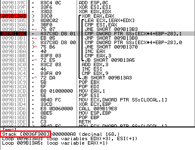
Fig. 7. Determining the address of the validation table
In my case, the table address is 0x36f308 (highlighted in red).
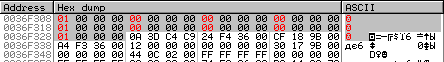
Fig. 8. Dump validation table
The search for the algorithm is performed in the same way that was demonstrated when solving the past of the crack, namely:
If everything was done correctly, you will find yourself here:

Fig. 9. Algorithm for filling the validation table
If you compare the new algorithm with the old one, you will notice that they differ:

Fig. 10. Old algorithm (screenshot from previous article )
The presentation of the "new algorithm" on Python is as follows:
Let us turn to the search for data used by this algorithm.
After analyzing the algorithm code, two places were found from which the data for its operation are taken:
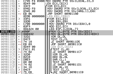
Fig. 11. Arrays with which the new algorithm operates
Above, they are highlighted by a gray rectangle. In my case, at addresses 0x9b11b0 and 0x9b11b2 , the following arrays are addressed:
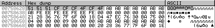
Fig. 12
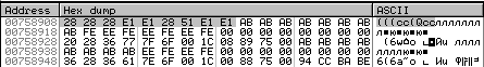
Fig. 13
Each array contains 9 elements one byte.
If we solved the old cracks, we would now go on to look for an algorithm for turning the serial code into an internal representation, but the new crack revealed a significant difference from the behavior of the old crack, so below is information about the differences that lie here.
In the old version of cracks, the work with the serial code was as follows:
In the end, we did something like this:
In the new version, everything is a little more complicated:
As a result, we get something like this:
From which it follows that we have a dependence on a fixed array .
I will leave the search for the serial code converter for you and I will not give it here. You can search in the same way as in the old version.
The table and the valid range are identical to the old version.
Now that all the necessary elements have been collected, you can proceed to the solution.
The algorithm of our actions is as follows:
If you read the first article , you probably remember that in order to compile the required table [1, 0, 0, 0, 1, 0, 0, 0, 1] , you need to have such bytes that when interacting with each other would give either " zeros " or " ones " .
In the old version of quacks, finding these bytes was very simple. All that had to be done was to go through the entire available alphabet and apply several simple operations to it.
In the new version it is much more difficult to do this (but this is only at first glance and I will explain why below). In the old version, we could iterate one item at a time. In the new version we have to sort through three elements, since all of them are interconnected.
Because in the first article I did not reveal that “magic”, which in reality was hidden behind the search for “zeros” and “ones” (in this article, it will have to be revealed, although it was possible not to do this). In my keygen, I used a function that looks for the required “zeros” and “ones”, but not in an entirely obvious way. This helped to successfully distract the most inquisitive and put them on the way of a single incident (which was the first crack). if they were given (like now) another crack, but with a different algorithm, they would have to invent a new way of searching for “zeros” and “ones”, which seems to happen to many;)
Well, okay, less words are more deeds.
Here is a magic “spell” that will help you find all null and single characters:

Fig. 14
Well, we have a group of elements giving "zeros" and "ones." How to get the desired table [1, 0, 0, 0, 1, 0, 0, 0, 1]?
The most attentive / shrewd ones might have noticed (for example, according to the comments to the previous article ) that we are dealing with matrices that, when multiplied by each other, should give the identity matrix [1, 0, 0, 0, 1, 0, 0, 0, one]. Therefore, to obtain the identity matrix, we need either two identity matrices, or two inverse ones.
To get the required unit matrix, you can use the following pattern:
Where in the place of y - substitute any single character, and instead of x - any zero.
You can use other patterns, you can find them using the following "spells":

Fig. 15
Having made a replacement, you can get, for example, such patterns:
Now, when we have dealt with obtaining the desired identity matrix (i.e. validation table), let's move on to other problems.
We know the following:
From which it follows that, for example, part_a depends on part_1 and salt . Which in turn narrows down the possible combinations for part_a . A natural question arises.
I think many have guessed what to do? That's right, use the next "spell"!
Here is one of them:
If your “spell” succeeds, you will see that only 4096 options are available for part_a and part_b (more precisely, “under options”).

Fig. sixteen
So now we have all the data to generate the first valid key. Of course, we should not forget that we work with bytes that have an internal representation, which means that before entering them into the window of a crack, they will still have to be reduced to a normal appearance.
If you were attentive, you probably noticed that all 4096 variants can be divided into two groups, those with “all elements are even” and those with “all elements are not even” .
index: 0035, table: [116, 222, 172] <= All elements are even
index: 0560, table: [172, 116, 222] <= All elements are even
index: 0770, table: [222, 172, 116] <= All elements are even
index: 0117, table: [1, 229, 111] <= All elements are not even
index: 1287, table: [229, 111, 1] <= All elements are not even
index: 1872, table: [111, 1, 229] <= All elements are not even
However, if you look at the “patterns” available to us, you will see that all of them require that each of the “options” have both “even” and “not even” elements, that is:
Here are two matrices that give us the identity:
part_a
[176, 176, 65] <= There are even and not even
[176, 65, 176] <= There are even and even
[65, 176, 176] <= There are even and even
part_b
[176, 176, 65] <= There are even and not even
[176, 65, 176] <= There are even and even
[65, 176, 176] <= There are even and even
valid_table = part_a * part_a
[ 100 ]
[0, 1, 0]
[0, 0, 1]
Since there are no “options” with “even” and “not even” elements, we conclude that there is an error in the quacks. There is a logical question.
After a quick reflection, we conclude that the error lies in the fixed matrix [0x3, 0x5, 0x7, 0x5, 0x7, 0x3, 0x7, 0x3, 0x5] . To get even and odd "options", you must replace "0x3" , "0x5" and "0x7" with "0x2" , "0x3" and "0x8", respectively, or with another variant, where there will be two even and one odd element, for example, on such "0x4" , "0x7" and "0x8" (as an option).
This error was reported to Kaspersky Lab. They said that the version (which we are currently exploring) is a draft. After that, on the same day, everyone was sent a version without error. True, in the new version, there were no fixed tables anymore and it was solved even easier than this one, but I will tell about this later in the bonus section :)
To make sure that you have performed the correct replacement (for example, if you decide to insert other characters other than "0x2" , "0x3" and "0x8" ), you should use the following "spell":
If the bait was chosen correctly (as in our case, “0x2, 0x3, 0x8”), then at least one beast (a group of three arrays) will appear in your traps (in the “Good” field). An example output for a fixed matrix (with the elements "0x2", "0x3" and "0x8") is shown below:

Fig. 17
As you can see, luck has smiled on us, so as many as three wild beasts fell into our traps, which of course will contribute to the setting of the holiday table (that is, it can be used to form part_a and part_b ).
The most attentive ones have already noticed that the output in the “Good” line can be divided into groups, each of which will have three lines.
[0, 144, 81]
[81, 0, 144]
[144, 81, 0]
[144, 145, 0]
[0, 144, 145]
[145, 0, 144]
[0, 144, 209]
[209, 0, 144]
[144, 209, 0]
Even more attentive probably noticed that all these characters are included in the sets of "zero" and "single" characters;)
Fig. 18
Well, the shrewd ones (I hope) are already feasting at the big table, as they were able to hunt down a big beast, luring it with such a “spell”:
At this point, we will finish solving this quack ... How to translate the internal bytes into a normal form, so that they can be entered into the window of the quack, I think you will understand.
For now you understand we will pass to consideration new (corrected) kryakmi. I just want to say that everything that we have considered for this quack is also relevant for the new, so we confine ourselves to a superficial description of the principle of its work and give a link to keygen (for the more curious or, on the contrary, lazy).
In order not to get confused with the available versions - we will introduce some clarity in their numbering:
As in all previous versions of v1 and v2 .
As in the draft version of v2 (discussed earlier in this article).
The principle of operation is the same as in the very first version of v1 , but other mixers are used.
As in all previous versions of v1 and v2 .
Cracks versions v2 and v3 can be found in this thread . There you will find the keygen for the new version v3 from me Darwin .
Password for archive from keygen: Darwin_1iOi7q7IQ1wqWiiIIw
Check keygen for the third version of crack:
> keygen_v3.py habrahabr.ru> result.txt
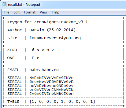
Fig. nineteen
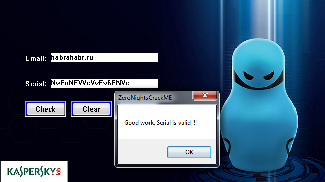
Fig. 20
Thanks to all who read to the end! See you soon!
On February 17, a letter arrived with a new quack. It is about his decision (and not only) that I will tell in this article.
Crack options are the same:
- File: ZeroNightsCrackMe.exe
- Platform: Windows 7 (64 bit)
- Packer: None
- Anti-debugging: Do not stumble
- Solution: Valid Mail / Serial Pair
Instruments:
- OllyDbg 2.01
- Some gray matter
Let's get down to solving ...
')
We go hunting
As usual, we run the test subject and perform a surface analysis. The reaction is similar to past quacks.
Fig. one
Knowing the principle of past quack work, let's start searching for key points and find:
- The function involved in processing the entered data.
- Algorithm validation table validation.
- Validation table
- Algorithm for filling the validation table.
- Data for the validation table filling algorithm.
- Algorithm of turning the serial code into an internal representation.
- Conversion table
- Valid range of characters.
After that, we will compare all key points with the previous version and find differences.
On animal tracks
Input processing function
First we find the function of processing the entered data. This is done quite simply. Click the right mouse button in the disassembler window and select “Search for => All referenced strings” :
Fig. 2
Next, click on the line "Good work, Serial is valid !!!" and get here:
Fig. 3
The above will be the desired function (in my case it is CALL 0x9b12b0 ). It is passed three parameters. In Arg2 , Arg1 , the size of the serial code and the pointer to the serial code are transmitted, respectively, and in the ECX register, the pointer is sent to the email.
Algorithm validation table validation
Go inside the function and turn to the bottom, there is an algorithm for checking the validation table (identical to the old version):
Fig. four
Validation Table Address
We set a breakpoint at the beginning of the algorithm and run cracks for execution (of course, first enter any data and click the Check button).
Fig. 5. Enter the test data
Fig. 6. Stop at the validation table
Now we define the address of the table itself. You can do this by going to the line “CMP DWORD PTR SS: [ECX * 4 + EBP-28], 1” and looking at the target address.
Fig. 7. Determining the address of the validation table
In my case, the table address is 0x36f308 (highlighted in red).
Fig. 8. Dump validation table
Algorithm for filling the validation table
The search for the algorithm is performed in the same way that was demonstrated when solving the past of the crack, namely:
- We continue the implementation of quacks (click F9 in Olka);
- We put bryak on the function of processing the entered data, in my case it is CALL 9b12b0 (Fig. 3);
- Switch to quacks and in the pop-up window (indicating success or non-success), click "OK" (thus continuing the work of the quacks);
- Next, click the "Check" button to start the recalculation of the serial, after which you should stop at the call CALL 0x9b12b0;
- Standing on the call CALL 0x9b12b0, put bryak on the record, at the address 0x36f308;
- And again press F9.
If everything was done correctly, you will find yourself here:
Fig. 9. Algorithm for filling the validation table
If you compare the new algorithm with the old one, you will notice that they differ:
Fig. 10. Old algorithm (screenshot from previous article )
The presentation of the "new algorithm" on Python is as follows:
def create_table(first_part, second_part): result = [] curr_second = 0 out_index = 0 while(out_index < 3): inner_index = 0 while(inner_index < 3): curr_first = 0 accumulator = 0 index = 0 while(index < 3): first = first_part[inner_index + curr_first] second = second_part[index + curr_second] hash = 0 if (first != 0): while (first != 0): if (first & 1): hash ^= second second += second first = first >> 1 accumulator ^= hash index += 1 curr_first += 3 result.append(accumulator & 0xff) inner_index += 1 out_index += 1 curr_second += 3 return result Let us turn to the search for data used by this algorithm.
Data for the validation table fill algorithm
After analyzing the algorithm code, two places were found from which the data for its operation are taken:
Fig. 11. Arrays with which the new algorithm operates
Above, they are highlighted by a gray rectangle. In my case, at addresses 0x9b11b0 and 0x9b11b2 , the following arrays are addressed:
- 0x00758628 (Fig. 12)
- 0x00758908 (Fig. 13)
Fig. 12
Fig. 13
Each array contains 9 elements one byte.
If we solved the old cracks, we would now go on to look for an algorithm for turning the serial code into an internal representation, but the new crack revealed a significant difference from the behavior of the old crack, so below is information about the differences that lie here.
The difference between the old version and the new one
In the old version of cracks, the work with the serial code was as follows:
- The serial code was broken into two parts.
- Each part was translated into an internal representation.
- Then each part was mixed (mixed).
- After that, both parts were transferred to the algorithm for filling the validation table.
In the end, we did something like this:
Serial |- part_1 |- part_2 part_1 = intermediate_view(part_1) part_2 = intermediate_view(part_2) part_1 = mix(part_1) part_2 = mix(part_2) valid_table = algo(part_1, part_2) In the new version, everything is a little more complicated:
- The serial code is divided into two parts.
- Each part of it is translated into an internal representation.
- The first part + fixed array (3, 5, 7, 5, 7, 3, 7, 3, 5) is passed to the algorithm.
- The second part + fixed array (3, 5, 7, 5, 7, 3, 7, 3, 5) is transferred to the algorithm.
- The result of points 3-4 is passed to the algorithm for filling the validation table.
As a result, we get something like this:
Serial |- part_1 |- part_2 part_1 = intermediate_view(part_1) part_2 = intermediate_view(part_2) part_1 = mix(part_1) part_2 = mix(part_2) salt = [3, 5, 7, 5, 7, 3, 7, 3, 5] part_a = algo(part_1, salt) part_b = algo(part_2, salt) valid_table = algo(part_a, part_b) From which it follows that we have a dependence on a fixed array .
Algorithm for turning the serial code into an internal representation
I will leave the search for the serial code converter for you and I will not give it here. You can search in the same way as in the old version.
Conversion table and valid range
The table and the valid range are identical to the old version.
Preparing a rookery for an ambush
Now that all the necessary elements have been collected, you can proceed to the solution.
The algorithm of our actions is as follows:
- For algo (part_a, part_b) , find such part_a and part_b , which give the result [1, 0, 0, 0, 1, 0, 0, 0, 1]
- For part_a = algo (part_1, salt) , find a part_1 that gives a result equal to part_a .
- For part_b = algo (part_2, salt) , find a part_2 that gives a result equal to part_b .
Let's start with algo (part_a, part_b)
If you read the first article , you probably remember that in order to compile the required table [1, 0, 0, 0, 1, 0, 0, 0, 1] , you need to have such bytes that when interacting with each other would give either " zeros " or " ones " .
In the old version of quacks, finding these bytes was very simple. All that had to be done was to go through the entire available alphabet and apply several simple operations to it.
In the new version it is much more difficult to do this (but this is only at first glance and I will explain why below). In the old version, we could iterate one item at a time. In the new version we have to sort through three elements, since all of them are interconnected.
And so, why does the new version seem complicated, but only at first glance?
Because in the first article I did not reveal that “magic”, which in reality was hidden behind the search for “zeros” and “ones” (in this article, it will have to be revealed, although it was possible not to do this). In my keygen, I used a function that looks for the required “zeros” and “ones”, but not in an entirely obvious way. This helped to successfully distract the most inquisitive and put them on the way of a single incident (which was the first crack). if they were given (like now) another crack, but with a different algorithm, they would have to invent a new way of searching for “zeros” and “ones”, which seems to happen to many;)
Well, okay, less words are more deeds.
Here is a magic “spell” that will help you find all null and single characters:
data_zero, data_ones = [], [] for a in range(0, 256): part_a = [a, a, a, a, a, a, a, a, a] part_b = [a, a, a, a, a, a, a, a, a] result = create_table(part_a, part_b) if result == [0, 0, 0, 0, 0, 0, 0, 0, 0]: data_zero.append(a) elif result == [1, 1, 1, 1, 1, 1, 1, 1, 1]: data_ones.append(a) print("ZERO:", data_zero) print("ONES:", data_ones) Fig. 14
Well, we have a group of elements giving "zeros" and "ones." How to get the desired table [1, 0, 0, 0, 1, 0, 0, 0, 1]?
The most attentive / shrewd ones might have noticed (for example, according to the comments to the previous article ) that we are dealing with matrices that, when multiplied by each other, should give the identity matrix [1, 0, 0, 0, 1, 0, 0, 0, one]. Therefore, to obtain the identity matrix, we need either two identity matrices, or two inverse ones.
To get the required unit matrix, you can use the following pattern:
# part_a = [y, x, x, x, y, x, x, x, y] part_b = [y, x, x, x, y, x, x, x, y] result = algo(part_a, part_b) Where in the place of y - substitute any single character, and instead of x - any zero.
You can use other patterns, you can find them using the following "spells":
happy = [1,32] for byte_1 in happy: for byte_2 in happy: for byte_3 in happy: for byte_4 in happy: for byte_5 in happy: for byte_6 in happy: for byte_7 in happy: for byte_8 in happy: for byte_9 in happy: part_1 = [byte_1, byte_2, byte_3, byte_4, byte_5, byte_6, byte_7, byte_8, byte_9] part_2 = [byte_1, byte_2, byte_3, byte_4, byte_5, byte_6, byte_7, byte_8, byte_9] result = create_table(part_1, part_2) if result == [1, 0, 0, 0, 1, 0, 0, 0, 1]: print("%s | %s " % (part_2, part_1)) Fig. 15
Having made a replacement, you can get, for example, such patterns:
patterns = [ # Pattern 0 [ [y1, x1, x1, x1, y2, x1, x1, x1, y3], [y1, x1, x1, x1, y2, x1, x1, x1, y3] ], # Pattern 1a [ [y1, x1, x1, x1, x1, y1, x1, y1, x1], [y1, x1, x1, x1, x1, y1, x1, y1, x1] ], # Pattern 1b [ [y1, x1, x2, x3, x4, y1, x5, y1, x6], [y1, x2, x1, x5, x6, y1, x3, y1, x4] ], # Pattern 2a [ [y1, x1, x1, x1, y1, x1, x1, x1, y1], [y1, x1, x1, x1, y1, x1, x1, x1, y1] ], # Pattern 2b [ [y1, x1, x2, x3, y2, x4, x5, x6, y3], [y1, x1, x2, x3, y2, x4, x5, x6, y3] ], # Pattern 3a [ [x1, x1, y1, x1, y1, x1, y1, x1, x1], [x1, x1, y1, x1, y1, x1, y1, x1, x1] ], # Pattern 3b [ [x1, x2, y1, x3, y2, x4, y3, x5, x6], [x6, x5, y3, x4, y2, x3, y1, x2, x1] ], # Pattern 4a [ [x1, y1, x1, y1, x1, x1, x1, x1, y1], [x1, y1, x1, y1, x1, x1, x1, x1, y1] ], # Pattern 4b [ [x1, y1, x2, y2, x3, x4, x5, x6, y3], [x3, y2, x4, y1, x1, x2, x6, x5, y3] ], # Pattern 5 [ [x1, x2, y1, y2, x3, x4, x5, y3, x6], [x4, y2, x3, x6, x5, y3, y1, x1, x2] ] ] Now, when we have dealt with obtaining the desired identity matrix (i.e. validation table), let's move on to other problems.
How to choose the appropriate part_a and part_b?
We know the following:
part_a = algo(part_1, salt) part_b = algo(part_2, salt) valid_table = algo(part_a, part_b) From which it follows that, for example, part_a depends on part_1 and salt . Which in turn narrows down the possible combinations for part_a . A natural question arises.
What combinations can we use?
I think many have guessed what to do? That's right, use the next "spell"!
Here is one of them:
# serial_data email “support@reverse4you.org” serial_data = [52, 233, 91, 105, 65, 15, 50, 176, 90, 40, 225, 81, 207, 79, 34, 19] def get_items(first_part, second_part): result = [] inner_index = 0 while(inner_index < 3): curr_first = 0 accumulator = 0 index = 0 while(index < 3): first = first_part[inner_index + curr_first] second = second_part[index] hash = 0 if (first != 0): while (first != 0): if (first & 1): hash ^= second second += second first = first >> 1 accumulator ^= hash index += 1 curr_first += 3 result.append(accumulator & 0xff) inner_index += 1 return result a = 0x3 b = 0x5 c = 0x7 first_part = [a, b, c, b, c, a, c, a, b] second_part_new = [0, 0, 0] count = 0 result_table = [] for byte_1 in serial_data: second_part_new[0] = byte_1 for byte_2 in serial_data: second_part_new[1] = byte_2 for byte_3 in serial_data: second_part_new[2] = byte_3 res = get_items(first_part, second_part_new) print("index: %s, table: %s" % (count, res)) count += 1 print("Count: %s" % count) If your “spell” succeeds, you will see that only 4096 options are available for part_a and part_b (more precisely, “under options”).
Fig. sixteen
So now we have all the data to generate the first valid key. Of course, we should not forget that we work with bytes that have an internal representation, which means that before entering them into the window of a crack, they will still have to be reduced to a normal appearance.
First victim (first valid key)
If you were attentive, you probably noticed that all 4096 variants can be divided into two groups, those with “all elements are even” and those with “all elements are not even” .
index: 0035, table: [116, 222, 172] <= All elements are even
index: 0560, table: [172, 116, 222] <= All elements are even
index: 0770, table: [222, 172, 116] <= All elements are even
index: 0117, table: [1, 229, 111] <= All elements are not even
index: 1287, table: [229, 111, 1] <= All elements are not even
index: 1872, table: [111, 1, 229] <= All elements are not even
However, if you look at the “patterns” available to us, you will see that all of them require that each of the “options” have both “even” and “not even” elements, that is:
Here are two matrices that give us the identity:
part_a
[176, 176, 65] <= There are even and not even
[176, 65, 176] <= There are even and even
[65, 176, 176] <= There are even and even
part_b
[176, 176, 65] <= There are even and not even
[176, 65, 176] <= There are even and even
[65, 176, 176] <= There are even and even
valid_table = part_a * part_a
[ 100 ]
[0, 1, 0]
[0, 0, 1]
Since there are no “options” with “even” and “not even” elements, we conclude that there is an error in the quacks. There is a logical question.
What is the mistake?
After a quick reflection, we conclude that the error lies in the fixed matrix [0x3, 0x5, 0x7, 0x5, 0x7, 0x3, 0x7, 0x3, 0x5] . To get even and odd "options", you must replace "0x3" , "0x5" and "0x7" with "0x2" , "0x3" and "0x8", respectively, or with another variant, where there will be two even and one odd element, for example, on such "0x4" , "0x7" and "0x8" (as an option).
This error was reported to Kaspersky Lab. They said that the version (which we are currently exploring) is a draft. After that, on the same day, everyone was sent a version without error. True, in the new version, there were no fixed tables anymore and it was solved even easier than this one, but I will tell about this later in the bonus section :)
To make sure that you have performed the correct replacement (for example, if you decide to insert other characters other than "0x2" , "0x3" and "0x8" ), you should use the following "spell":
serial_data = [52, 233, 91, 105, 65, 15, 50, 176, 90, 40, 225, 81, 207, 79, 34, 19] a = 0x2 b = 0x3 c = 0x8 first_part = [a, b, c, b, c, a, c, a, b] second_part_new = [0, 0, 0] count = 0 result_table = [] for byte_1 in serial_data: second_part_new[0] = byte_1 for byte_2 in serial_data: second_part_new[1] = byte_2 for byte_3 in serial_data: second_part_new[2] = byte_3 res = get_items(first_part, second_part_new) print("index: %s, table: %s" % (count, res)) if (res[0] % 16 == 0 and res[1] % 16 == 0 and res[2] % 16 == 1) or\ (res[0] % 16 == 1 and res[1] % 16 == 0 and res[2] % 16 == 0) or\ (res[0] % 16 == 0 and res[1] % 16 == 1 and res[2] % 16 == 0): result_table.append(res) count += 1 print("Count:", count) print("Good:", result_table) If the bait was chosen correctly (as in our case, “0x2, 0x3, 0x8”), then at least one beast (a group of three arrays) will appear in your traps (in the “Good” field). An example output for a fixed matrix (with the elements "0x2", "0x3" and "0x8") is shown below:
Fig. 17
As you can see, luck has smiled on us, so as many as three wild beasts fell into our traps, which of course will contribute to the setting of the holiday table (that is, it can be used to form part_a and part_b ).
The most attentive ones have already noticed that the output in the “Good” line can be divided into groups, each of which will have three lines.
[0, 144, 81]
[81, 0, 144]
[144, 81, 0]
[144, 145, 0]
[0, 144, 145]
[145, 0, 144]
[0, 144, 209]
[209, 0, 144]
[144, 209, 0]
Even more attentive probably noticed that all these characters are included in the sets of "zero" and "single" characters;)
Fig. 18
Well, the shrewd ones (I hope) are already feasting at the big table, as they were able to hunt down a big beast, luring it with such a “spell”:
# # [0, 144, 209] # [209, 0, 144] # [144, 209, 0] a = 144 b = 209 c = 0 # part_a = [c, a, b, b, c, a, a, b, c] part_b = [a, b, c, c, a, b, b, c, a] # part_a1 = [0, 144, 209] # part_a2 = [209, 0, 144] # part_a3 = [144, 209, 0] # part_a = part_a1 + part_a2 + part_a3 # part_b1 = [144, 209, 0] # part_b2 = [0, 144, 209] # part_b3 = [209, 0, 144] # part_b = part_b1 + part_b2 + part_b3 result = create_table(part_a, part_b) print(result) At this point, we will finish solving this quack ... How to translate the internal bytes into a normal form, so that they can be entered into the window of the quack, I think you will understand.
For now you understand we will pass to consideration new (corrected) kryakmi. I just want to say that everything that we have considered for this quack is also relevant for the new, so we confine ourselves to a superficial description of the principle of its work and give a link to keygen (for the more curious or, on the contrary, lazy).
Bonus (keygen + new crack job description)
In order not to get confused with the available versions - we will introduce some clarity in their numbering:
- ZeroNightsCrackMe_v1 - reviewed here .
- ZeroNightsCrackMe_v2 - is a draft version and is described earlier in this article.
- ZeroNightsCrackMe_v3 - superficially discussed below + given keygen.
The validation table check algorithm and the validation table itself
As in all previous versions of v1 and v2 .
Algorithm for filling the validation table
As in the draft version of v2 (discussed earlier in this article).
Data for algortim filling validation table
The principle of operation is the same as in the very first version of v1 , but other mixers are used.
Algorithm for converting a serial code into an internal representation, a conversion table and an allowable range
As in all previous versions of v1 and v2 .
Keygen for the new version
Cracks versions v2 and v3 can be found in this thread . There you will find the keygen for the new version v3 from me Darwin .
Password for archive from keygen: Darwin_1iOi7q7IQ1wqWiiIIw
Check keygen for the third version of crack:
> keygen_v3.py habrahabr.ru> result.txt
Fig. nineteen
Fig. 20
Thanks to all who read to the end! See you soon!
Source: https://habr.com/ru/post/215225/
All Articles