Implementing BFS Algorithm on GPU

annotation

In this article I want to tell how you can effectively parallelize the algorithm BFS - search in width in the graph using graphics accelerators. The article will provide a detailed analysis of the algorithm. The calculations were performed on a single GPU GTX Titan Kepler architecture.

Introduction

Recently, graphic accelerators (GPU) in non-graphical calculations play an increasing role. The need for their use is due to their relatively high performance and lower cost. As you know, on a GPU, tasks on structural grids are well solved, where parallelism is somehow easily distinguished. But there are tasks that require high power and use non-structural grids. An example of such a task is the Single Shortest Source Path problem (SSSP) - the task of finding the shortest paths from a given vertex to all others in a weighted graph. The solution to this problem is considered by me in this article. The second example of a problem on nonstructural grids is the Breadth First Search (BFS) problem — a wide search in an undirected graph. This task is fundamental in a number of algorithms on graphs. It is also a bit simpler than finding the shortest path. At the moment, the BFS algorithm is used as the main test for the Graph500 rating. Next, we consider how to use the ideas of solving the SSSP problem in the BFS problem. Nvidia’s GPU architecture and the mentioned algorithms have already been written a lot, so in this article I will not write further about it. Also, I hope that the concepts of warp, cuda block, SMX, and other basic things related to CUDA are familiar to the reader.

The format of the data used

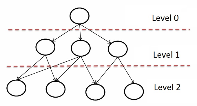
Just like in the SSSP task, we will use the same transformations in order to increase the load on one SMX and reduce the amount of identical data stored in the global memory of the GPU. The main difference is that the BFS algorithm does not need weights in the graph. It is also worth noting that we need to store not the shortest distances, but the number of the level at which this vertex is located:


')
After the test launches, it turned out that the number of levels in RMAT graphs with an average degree of connectivity 32 does not exceed 10. Therefore, unsigned char will be enough to store the data values. Thus, the array of levels will occupy 8 times less space than the array of distances, which is very important, since the cache size in the Kepler architecture is only 1.5 MB.

The implementation of the algorithm on the CPU

On the CPU, a native version of the wide bypass algorithm was implemented, namely the creation of a queue of not yet viewed vertices. The implementation CPU code looks like this:

queue<vertex_id_t> q; bool *used = new bool[G->n]; for (unsigned i = 0; i < G->n; ++i) used[i] = false; used[root] = true; q.push(root); dist[root] = 0; while (!q.empty()) { vertex_id_t nextV = q.front(); q.pop(); for (unsigned k = G->rowsIndices[nextV]; k < G->rowsIndices[nextV + 1]; ++k) { if (used[G->endV[k]] == false) { used[G->endV[k]] = true; q.push(G->endV[k]); dist[G->endV[k]] = dist[nextV] + 1; } } } 

This code is quite simple and, quite possibly, not optimal. It was used to verify the correct operation of the algorithm on the GPU. There were no goals to write the optimal algorithm on the CPU, so the performance on the CPU will be obtained by this algorithm. I want to add that at the moment optimal CPU implementations are many and easy to find. Also proposed are many other approaches and ideas for implementing the BFS algorithm.

The implementation of the algorithm on the GPU

The implementation was based on the same Ford-Bellman algorithm and core in the SSSP problem considered. The main computational core for BFS will look like this:

 if(k < maxV) { unsigned en = endV[k]; unsigned st = startV[k]; if(levels[st] == iter) { if(levels[en] > iter) { levels_NR[en] = iter + 1; modif[0] = iter; } } else if(levels[en] == iter) { if(levels[st] > iter) { levels_NR[st] = iter + 1; modif[0] = iter; } } } 

The idea of ​​the algorithm is as follows. Let the levels array be initially filled with the maximum value for the selected type (255 for unsigned char). We will transfer the current iteration number to the kernel - iter. Next, you need to look through all the edges and check whether the starting or ending vertex is the current parent, that is, it belongs to the iter level. If yes, then it is necessary to mark the opposite vertex of the arc being viewed with a value one more to “include” this vertex in the list of parents at the next iteration. As well as in SSSP, the variable modif remains, indicating the need to continue marking the graph.
This code already contains the applied optimizations in the SSSP task — using const __restrict for the levels array and using another levels_NR reference pointing to the same memory location needed for recording. The second permutation optimization for better data localization in the cache was also used. For the BFS algorithm, the length of the optimal cache line is 1024KB, or about 1 million elements of the levels array (1024 * 1024), regardless of the size of the graph.

Analysis of the results

For testing, we used synthetic undirected RMAT-graphs, which simulate real graphs from social networks and the Internet well. The graphs have an average connectivity of 32, the number of vertices is a power of two. The table below shows the columns on which the testing was conducted:

Number of vertices 2 ^ N	Number of vertices	Number of arcs	Array size in MB	MB edge array size
14	16 384	524 288	> 0.125	2
15	32,768	1,048,576	> 0.125	four
sixteen	65,536	2,097,152	> 0.125	eight
17	131,072	4 194 304	0.125	sixteen
18	262 144	8,388,608	0,250	32
nineteen	524 288	16 777 216	0.5	64
20	1,048,576	33,554,432	one	128
21	2,097,152	67 108 864	2	256
22	4 194 304	134 217 728	four	512
23	8,388,608	268 435 456	eight	1024
24	16 777 216	536 870 912	sixteen	2048

Due to the use of the smallest data type for storing level values, for a graph with a number of vertices of 2 ²⁰ , 1MB is needed for caching the array of levels, while for the same graph in the SSSP task, 8MB is needed. Testing was carried out on the NVidia GTX Titan GPU, which has 14 SMX and 2688 CUDA cores and a 3rd generation Intel core i7 processor with a frequency of 3.4 GHz and 8 MB of cache. To compare the performance on the CPU, a native implementation of the search algorithm was used. No optimizations in the form of data swapping before working on the CPU were made. Instead of time, we consider the number of arcs processed per second of time as a measure of performance. In this case, it is necessary to divide the time received by the number of arcs in the graph. As an end result, an average value of 32 points was taken. Also calculated the maximum and minimum values. The compilers used were Intel 13th compilers and NVCC CUDA 5.5 with the –O3 –arch = sm_35 flags.

The graph of the average performance of the various options on the GPU and CPU is as follows:



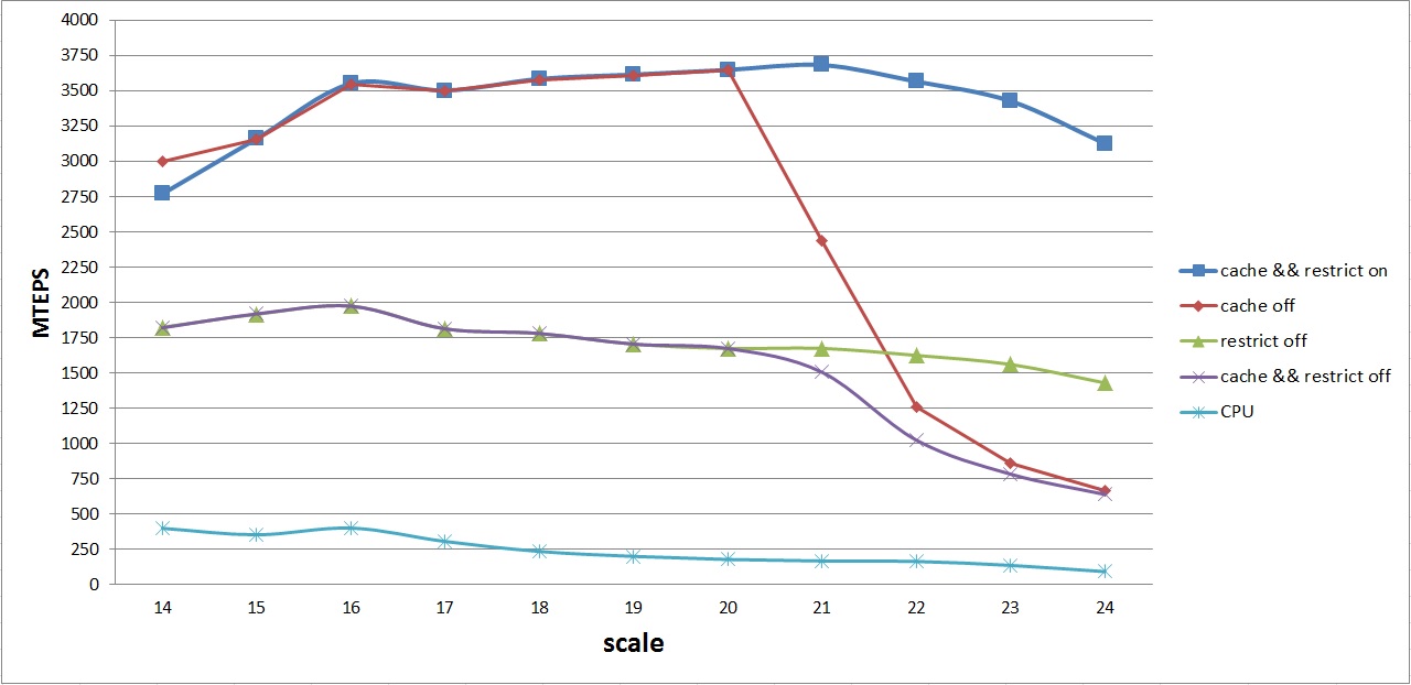
This graph shows the average performance curves for the following algorithms:

• cache && restrict on - GPU algorithm with all optimizations (1)
• cache off - GPU algorithm without optimizing permutations for improved caching (2)
• restrict off - GPU algorithm without texture cache optimization (3)
• cache && restrict off - basic GPU algorithm without optimizations (4)
• CPU - the basic algorithm on the CPU

The first thing that catches the eye is the identical behavior of algorithms (1) - (2) and (3) - (4). As noted above, this is due to the fact that the levels array for graphs with the number of vertices up to 2 ²⁰ is placed in the L2 cache. Therefore, you can not make a permutation of the arcs, if we consider the algorithms (1) and (2), and do not use the texture cache in case (3) and (4).

Further, it can be noted that as soon as the levels array does not fit in the L2 cache, disabling the permutation gives a strong performance loss, despite the fact that const __restrict is used. This is primarily due to random access to the levels array. A similar picture is observed in the case of disabling the option const __restirict.

Not a smooth graph in the range of degrees 15-16-17 for the best algorithm is the result of another small optimization - packing two vertices of one arc into one variable of unsigned int type. Since the maximum vertex number is 16 bits, and unsigned int is 32 bits, you can pack the edge data in one unsigned int in advance, and unpack it in the kernel, reading two times less than the data from the global memory of the GPU.

As a result, the average performance of 3.6 GTEPS was achieved. Almost peak average performance is achieved on graphs with the number of vertices 2 ¹⁶ - 2 ²³ , which is not bad enough for this architecture. Maximum performance is obtained on a graph with the number of vertices 2 ¹⁹ - 4.2 GTEPS.

The resulting acceleration compared to the native implementation on the CPU was not very clear:



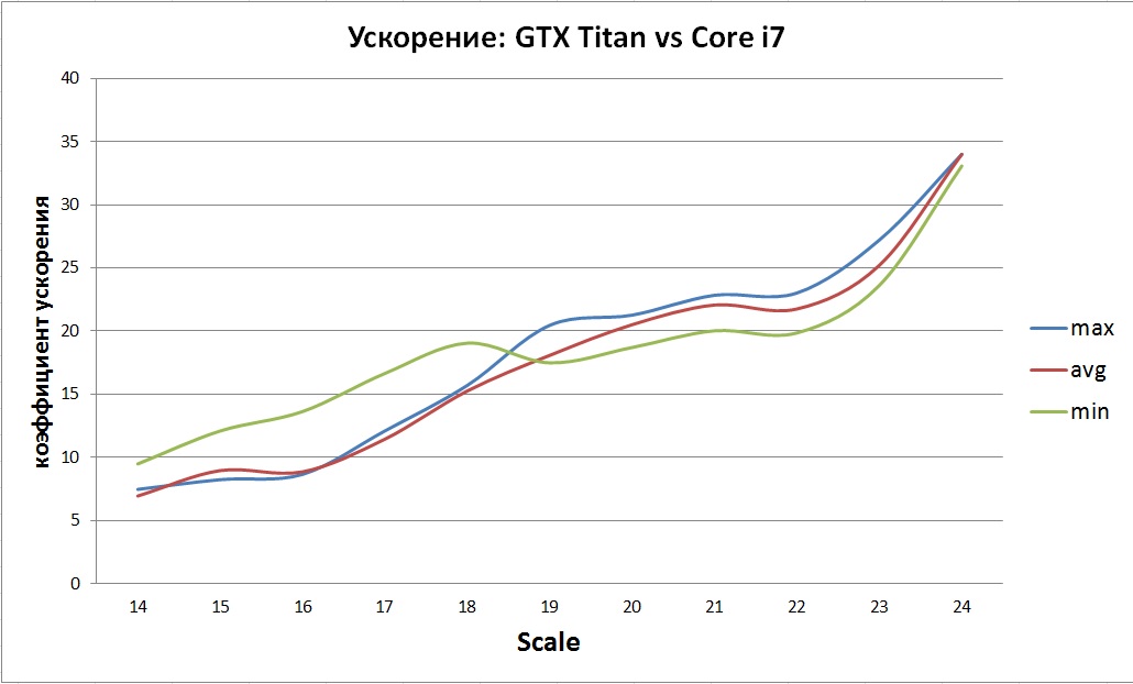
The general trend is visible - a gradual increase in acceleration. Most likely this is due to inefficient implementations and limited CPU cache size.

Detailed analysis of the implemented kernel

In conclusion, I would like to show how effective this approach is in terms of the use of GPU resources. This section is presented only for interest and, perhaps, for those who in the future will want to compare their algorithm with what is presented in this article. Let us consider in detail all that the NVVP profiler displays for two graphs - 2 ¹⁹ and 2 ²² . I chose such graphs, because the first level array completely fits into the L2 cache, and the second one does not. In the beginning we will consider general information:

Scale	Number of iterations performed	Shared Memory Usage	Number of registers used	Total kernel count time in ms	Array copy time in ms
2 19	7	not	12	4,512	10.97
2 22	eight	not	12	41.1	86.66

Taking into account the copying of arrays of vertices on the GPU before the start of the counting and copying the result on the CPU after the end From the table it can be seen that copying takes approximately twice as long as the entire bill. Next, consider the iterations for each graph.

Count 2 ¹⁹

Iteration	Time in ms	GL Eff,%	GS Eff,%	WE Eff,%	NP WE Eff,%	Occupancy,%	L2 Read, GB / s	L2 Write, GB / s	Global Read, GB / s	Global Write, GB / s
one	0.577	100	ten	100	94.6	89.3	551	0.0002	110	0.0002
2	0.572	100	8.1	99.9	94.5	89.2	551	0.0986	110	0.0498
3	0.58	100	11.9	93.5	88.5	88.1	545	14	109	6
four	1.062	100	24.3	85.1	77.7	78.2	289	71	58	51
five	0.576	100	9.5	91.1	86.8	88.8	549	1.37	110	0.5576
6	0.576	100	7,8	99.6	94.2	89.2	551	0.0017	110	0.0010
7	0.572	100	0	100	94.6	89.3	551	0.000	110	0.000

Decryption:

• GL Eff - Global Load Efficiency
• GS Eff - Global Store Efficiency
• WE Eff - Warp Execution efficiency
• NP WE Eff - Non-predicated Warp Execution efficiency
• Occupancy - the number of real active warps / maximum number of warps on SMX

From the table it can be seen that the largest number of vertices is processed at 3 and 4 iterations. Because of this, at the 4th iteration, a decrease in the use of L2 bandwidth and global GPU memory is visible. It should be noted that according to the specifics of the algorithm, no entries occur at the last iteration. It is necessary to determine the completeness of the graph layout. Efficiency of execution of warps is within 93-100% and 85% at the most "loaded" iteration.
For comparison, below is a table for a graph with 2 ²² vertices, the size of whose levels array does not fit entirely into the L2 GPU cache.

Count 2 ²²

Iteration	Time in ms	GL Eff,%	GS Eff,%	WE Eff,%	NP WE Eff,%	Occupancy,%	L2 Read, GB / s	L2 Write, GB / s	Global Read, GB / s	Global Write, GB / s
one	4.66	100	10.4	100	94.6	89.1	556	0.0001	113	0.00001
2	4.60	100	11.8	100	94.6	89.1	556	0.0014	113.2	0,0011
3	4.61	100	11.2	99.8	94.4	89.1	555	0.5547	117	0.3750
four	6,405	100	17,8	83.7	79.1	82.2	399	46	81	28
five	7,016	100	15.8	83.6	74.1	79.8	364	34	74	nineteen
6	4.62	100	7.9	90.2	85,5	89.1	555	0.0967	117	0.0469
7	4.60	100	7,8	100	94.6	89	556	0.0002	113	0.0001
eight	4.60	100	0	100	94.6	89.1	556	0.000	113	0.000

Decoding is given above. This graph shows approximately the same picture as on 2 ¹⁹ . The peak is at 4-5 iterations. According to the NVVP profiler, the L2 cache capacity of 560 GB / s is high (there is low, medium, high, maximum), and the global memory of 117 GB / s is medium (there is low, medium, high, maximum).

Conclusion

As a result of the work done, a wide search algorithm was implemented and optimized on RMAT graphs with an average degree of connectivity of vertices 32. A peak performance of 4.2 GTEPS and an average of 3.6 GTEPS was achieved. As you know, not only performance is important, but also energy efficiency. Along with the Graph500 rating, there is a Green Graph500 rating showing energy efficiency. The first place in the Graph500 performance rating for March 2014 is occupied by BlueGene / Q, Power BQC 16C 1.60 GHz with the number of cores 1048576 and the number of nodes 65536 with a capacity of 15363 GTEPS. The power consumption of such a system is 340kW (taken from the top 500 rating). The efficiency of the GTEPS / kW result for BlueGene / Q is 45. For the algorithm implemented by me, we get about 18 (the total power of 200W and the average performance of 3.6 GTEPS were taken for the calculation, since only one 4x CPU core is involved in the work and the peak load on the GPU is not achieved).
I would also like to note that in the Graph500 rating there is a similar Xeon E5-2650 v2 system, the GeForce GTX TITAN, which in the 2 ²⁵ column received a performance of 17 GTEPS. Unfortunately, information about which graph was used is not given. As of March 2014, this system is at 58 positions in the ranking.