Implementing SSSP Algorithm on GPU

annotation

In this article I want to tell you how you can effectively parallelize the algorithm SSSP - search for the shortest path in the graph using graphics accelerators. The GTX Titan Kepler architecture map will be considered as a graphics accelerator.

Introduction

Recently, graphic accelerators (GPU) in non-graphical calculations play an increasing role. The need for their use is due to their relatively high performance and lower cost. As you know, on a GPU, tasks on structural grids are well solved, where parallelism is somehow easily distinguished. But there are tasks that require high power and use non-structural grids. An example of such a task is the Single Shortest Source Path problem (SSSP) - the task of finding the shortest paths from a given vertex to all others in a weighted graph. To solve this problem, there are at least two well-known algorithms on the CPU: the Actionctry algorithm and the Ford-Bellman algorithm. There are also parallel implementations of the Deistra and Ford-Bellman algorithm on the GPU. Here are the main articles that describe the solution to this problem:

1. Accelerating Large Graph Algorithms for GPU Using CUDA, Pawan Harish and PJ Narayanan
2. A New GPU-based Approach to the Shortest Path Problem, Orchega-Arranz Hector, Yuri Torres, Diego R. Llanos, and Arturo Gonzalez-Escribano

There are other English-language articles. But in all these articles the same approach is used - the idea of ​​the algorithm of Diskra. I will describe how you can use the idea of ​​the Ford-Bellman algorithm and the advantages of the Kepler architecture to solve the problem. A lot has been written about the GPU architecture and the mentioned algorithms, so in this article I will not additionally write about it. Also, it is believed that the concepts of warp (warp), cuda block, SMX, and other basic things related to CUDA are familiar to the reader.

Description of the data structure

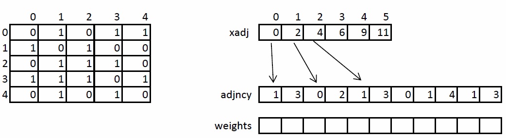
We briefly consider the storage structure of an undirected weighted graph, since in the future it will be mentioned and transformed. The graph is set in compressed CSR format. This format is widely used to store sparse matrices and graphs. For a graph with N vertices and M edges, three arrays are needed: xadj, adjncy, weights. The xadj array of size N + 1, the remaining two - 2 * M, since in the undirected graph for any pair of vertices it is necessary to store the forward and reverse arcs.

The principle of storage of the graph is as follows. The entire list of neighbors of vertex I is in the adjncy array from index xadj [I] to xadj [I + 1], not including it. For similar indices, weights of each edge from vertex I are stored. For the illustration, the graph on the left shows a graph of 5 vertices, recorded using an adjacency matrix, and on the right, in CSR format.
')

The implementation of the algorithm on the GPU

Input preparation

In order to increase the computational load on a single stream multiprocessor (SMX), it is necessary to convert the input data. All conversions can be divided into two stages:

• Expansion of CSR format to coordinate format (COO)
• Sort COO format

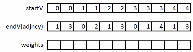
At the first stage, it is necessary to expand the CSR format as follows: we will introduce another startV array in which we will store the beginnings of the arcs. Then their ends will be stored in the adjncy array. Thus, instead of storing neighbors, we will store arcs. An example of this transformation on the graph described above:



At the second stage, it is necessary to sort the obtained edges so that each pair (U, V) occurs exactly once. Thus, when processing the edge (U, V), you can immediately process the edge (V, U) without re-reading the data about this edge from the global memory of the GPU.

Core Computing Core

The Ford-Bellman algorithm was taken as the basis for implementation on the GPU. This algorithm is well suited for implementation on a GPU due to the fact that the edges can be viewed independently of each other and the data of the edges and their weights are arranged in a row, which improves the throughput of the GPU memory:

int k = blockIdx.x * blockDim.x + threadIdx.x; if(k < maxV) { double w = weights[k]; unsigned en = endV[k]; unsigned st = startV[k]; if(dist[st] > dist[en] + w) // (*) { dist[st] = dist[en] + w; modif[0] = iter; } else if(dist[en] > dist[st] + w) // (**) { dist[en] = dist[st] + w; modif[0] = iter; } } 

In this core, each thread processes two edges (forward and reverse), trying to improve the distance along one of them. It is clear that both conditions of the if block cannot be fulfilled simultaneously. Unlike the Ford-Bellman algorithm, where each edge is scanned sequentially, a situation of “race” of flows can occur in the algorithm implemented on the GPU — when two or more streams enter to update the same cell dist [I]. We show that in this case the algorithm will remain correct.

Suppose there are two threads K1 and K2 that want to update the cell dist [I]. This means that the condition (*) or (**) is fulfilled. Two cases are possible. The first is one of the two threads recorded the smallest value. Then at the next iteration for these two threads the condition will be false, and the value in the dist [I] cell will be minimal. The second - one of the two threads recorded not the minimum value. Then at the next iteration the condition will be true for one of the threads, and false for the other. Thus, the result will be the same in both cases, but achieved in a different number of iterations.

According to the optimized version of the Ford-Bellman algorithm, if at any iteration there were no changes in the dist array, then it does not make sense to iterate further. For these purposes, the variable modif was introduced on the GPU, in which the threads recorded the current iteration number.

One iteration - one launch of the kernel. In the base case, we start the kernel on the CPU in a cycle, then read the modif variable and, if it has not changed from the previous iteration, then in the dist array the answer of the problem is the shortest path from the specified vertex to all others.

Optimization of the implemented algorithm

Next, we consider some optimizations that can significantly improve the performance of the algorithm. Knowledge of the final architecture can be useful when performing optimizations.

Modern CPUs have a three-level cache. The size of the first-level cache is 64KB and is contained on all the processing cores of the processor. The size of the second level cache varies from 1 to 2MB. The cache of the third level is common to the entire CPU and has a size of about 12-15MB.

Modern GPUs have a two-level cache. The size of the first level cache is 64KB. Used for shared memory and forcing out registers. For shared memory is available no more than 48KB. Contained in each computing unit. The maximum cache size in the second level is 1.5 MB and is common to the entire GPU. Used to cache data loaded from the GPU's global memory. In the most modern GPU chip GK110 there are 15 computing units. It turns out that one block has approximately 48KB of the first-level cache and 102KB of the second-level cache. Compared to the CPU, it is very small, so reading from the global memory of the graphics processor is more expensive than from the main memory of the CPU. Also, the Kepler architecture has the ability to directly access the read-only texture cache. To do this, you must add in the kernel before the corresponding formal parameter const __restrict.

Texture Cache Usage

In this task, you need to constantly update and read the distance array dist. This array takes up quite a bit of space in the global memory of the GPU compared to information about arcs and their weights. For example, for a graph with the number of vertices 2 ²⁰ (approximately 1 million), the dist array will occupy 8MB. Despite this, access to this array is carried out randomly, which is bad for the GPU, since additional loads are generated from global memory to each computational warp. In order to minimize the number of downloads per warp, it is necessary to store data in the L2 cache, read but not used data by other warp.

Since the texture cache is read-only, in order to use it, I had to enter two different references to the same dist distance array. Corresponding code:

 __global__ void relax_ker (const double * __restrict dist, double *dist1, … …) { int k = blockIdx.x * blockDim.x + threadIdx.x + minV; if(k < maxV) { double w = weights[k]; unsigned en = endV[k]; unsigned st = startV[k]; if(dist[st] > dist[en] + w) { dist1[st] = dist[en] + w; modif[0] = iter; } else if(dist[en] > dist[st] + w) { dist1[en] = dist[st] + w; modif[0] = iter; } } } 

As a result, it turned out that inside the kernel all read operations are carried out with one array, and all write operations with another. But both dist and dist1 links point to the same section of GPU memory.

Localize data to better use cache

For the best optimization work described above, it is necessary that as long as possible the downloaded data is in the L2 cache. Access to the dist array is carried out using predefined indices stored in the endV and startV arrays. To localize the calls, we divide the dist array into segments of a certain length, for example, P elements. Since there are only N vertices in the graph, we obtain (N / P + 1) different segments. Next, we will re-sort the edges into these segments as follows. In the first group we assign the edges, the ends of which fall into the zero segment, and the beginning - first in the zero, then in the first, etc. In the second group we assign the edges, the ends of which fall into the first segment, and the beginning - first in the zero, then in the first, etc.

After a given permutation of the edges, the values ​​of the elements of the dist array, corresponding to, for example, the first group, will be in the cache as long as possible, since the threads in the first group will request data from the zero segment for leaf vertices and zero, the first, etc. for initial vertices. Moreover, the edges are arranged so that the threads will request data from no more than three different segments.

Algorithm Test Results

For testing, we used synthetic undirected RMAT-graphs , which simulate real graphs from social networks and the Internet well. The graphs have an average connectivity of 32, the number of vertices is a power of two. The table below shows the columns on which the testing was conducted.

Number of vertices 2 ^ N	Number of vertices	Number of arcs	Dist array size in MB	Size of arrays of ribs and weights in MB
14	16 384	524 288	0.125	four
15	32,768	1,048,576	0,250	eight
sixteen	65,536	2,097,152	0,500	sixteen
17	131,072	4 194 304	one	32
18	262 144	8,388,608	2	64
nineteen	524 288	16 777 216	four	128
20	1,048,576	33,554,432	eight	256
21	2,097,152	67 108 864	sixteen	512
22	4 194 304	134 217 728	32	1024
23	8,388,608	268 435 456	64	2048
24	16 777 216	536 870 912	128	4096

The table shows that an array of distances dist for a graph with the number of vertices 2 ¹⁸ and more does not fit entirely into the L2 cache on the GPU. Testing was done on the Nividia GTX Titan GPU, which has 14 SMX with 192 cuda cores (2688 in total) and the 3rd generation Intel core i7 processor with a frequency of 3.4 GHz and 8 MB of cache. To compare the performance on the CPU, an optimized Dijkstra algorithm was used. No optimizations in the form of data swapping before working on the CPU were made. Instead of time, we consider the number of arcs processed per second of time as a measure of performance. In this case, it is necessary to divide the time received by the number of arcs in the graph. As an end result, an average value of 32 points was taken. The maximum and minimum values ​​were also calculated.

The compilers used were Intel 13th compilers and NVCC CUDA 5.5 with the –O3 –arch = sm_35 flags.

As a result of the work done, consider the following graph:



This graph shows the average performance curves for the following algorithms:

1. cache && restrict on - GPU algorithm with all optimizations
2. cache off - GPU algorithm without optimizing permutations for improved caching
3. restrict off - GPU algorithm without texture cache optimization
4. cache && restrict off - basic GPU algorithm without optimizations
5. CPU - the basic algorithm on the CPU

It can be seen that both optimizations strongly affect performance. It is worth noting that incorrect use of const __restrict optimization can degrade performance. The resulting acceleration can be seen in this graph:



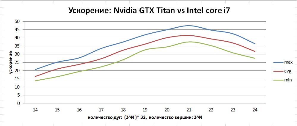
The graph shows that, unlike the CPU, the GPU has a larger range of deviations from the average. This is due to the peculiarity of the implementation of the algorithm in the form of a “race” of threads, since we can get a different number of iterations from launch to launch.

Conclusion

As a result of the work done, the SSSP algorithm, the search for the shortest paths in a graph, was developed, implemented and optimized. This algorithm searches for the shortest distances in a graph from a given vertex to all the others. Among all the graphs that fit in the GTX Titan memory, the maximum performance is shown by graphs with the number of peaks up to 2 ²¹ - about 1100 million edges per second. The maximum average acceleration that was achieved was about 40 on graphs with the number of vertices from 1 to 4 million.

Literature

1. CUDA
2. Graph
3. Ford-Bellman algorithm
4. Dijkstra's basic algorithm