Applying a Poisson transform for seamless image overlay
In tasks of machine vision and automated image processing, the task of seamless overlay of images is often encountered. For clarity, just give an example.
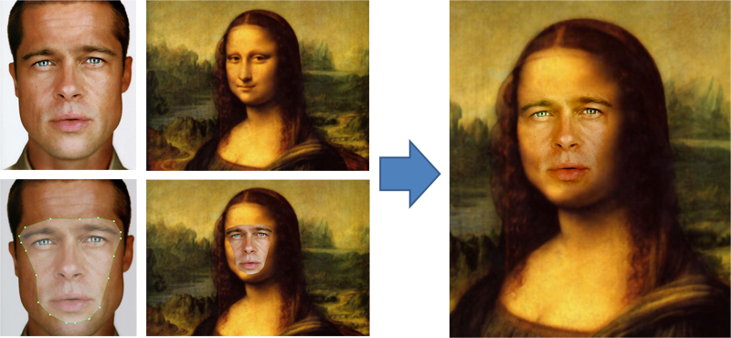
A seamless overlay of images (blending) will be called a method that allows you to insert a part of one image into another so that there are no noticeable seams on the borders of the inserted image. This method adjusts the inserted part to the rest of the image. In fact, to get the result, only the gradient field of the inserted part and the pixel values of the original image on the border of the processed area are used.
Suppose we have images A on which image B is superimposed in a certain place.
')
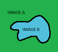
For seamless blending, it is necessary that the gradient of the image A in the area of the image B be equal to the gradient of the image B. The color restoration on the area B will be based on the gradient in the area B and the data about the color of the image A on the border of the area B.
This means that to get the resulting image, you must restore the image by its gradient, i.e. solve the Poisson problem.
Below is a solution to the problem for the monotonous image. For RGB image method is applied to each channel.
We define the boundary of the inserted area as follows:

And calculate the gradient of the overlay image:

Now all the data is available and we can make up the Poisson equation:

where (x, y) is the current pixel coordinate, N is the number of neighboring pixels not including borders (no more than 4), (dx, dy) are coordinates of neighboring pixels, can take values from the set {(-1, 0), (1 , 0), (0, -1), (0, 1)}
Thus, an equation is compiled for each unknown pixel. As a result, we get a system with M unknowns, where M is the number of pixels of the inserted image. It remains only to solve this system. There are quite a few methods for solving this problem, but the Jacobi method and the Gauss – Seidel method are usually used for the solution.
Often, a gradient field is mixed in the overlay area with the original image. For example, take the maximum value of gradients A or B at a certain point. It is best to feel the difference between the original and combined gradient by example.
Image gradient recovery:

Recovery by the maximum gradient of images A and B:
It is obvious that it is advisable to apply image recovery by a combined gradient for objects that have a transparent structure (water, rainbow, clouds, etc.).

But what would a rainbow look like without a combination of gradients

A seamless overlay of images (blending) will be called a method that allows you to insert a part of one image into another so that there are no noticeable seams on the borders of the inserted image. This method adjusts the inserted part to the rest of the image. In fact, to get the result, only the gradient field of the inserted part and the pixel values of the original image on the border of the processed area are used.
Formulation of the problem
Suppose we have images A on which image B is superimposed in a certain place.
')
For seamless blending, it is necessary that the gradient of the image A in the area of the image B be equal to the gradient of the image B. The color restoration on the area B will be based on the gradient in the area B and the data about the color of the image A on the border of the area B.
This means that to get the resulting image, you must restore the image by its gradient, i.e. solve the Poisson problem.
Below is a solution to the problem for the monotonous image. For RGB image method is applied to each channel.
Decision
We define the boundary of the inserted area as follows:
And calculate the gradient of the overlay image:
Now all the data is available and we can make up the Poisson equation:
where (x, y) is the current pixel coordinate, N is the number of neighboring pixels not including borders (no more than 4), (dx, dy) are coordinates of neighboring pixels, can take values from the set {(-1, 0), (1 , 0), (0, -1), (0, 1)}
Thus, an equation is compiled for each unknown pixel. As a result, we get a system with M unknowns, where M is the number of pixels of the inserted image. It remains only to solve this system. There are quite a few methods for solving this problem, but the Jacobi method and the Gauss – Seidel method are usually used for the solution.
Often, a gradient field is mixed in the overlay area with the original image. For example, take the maximum value of gradients A or B at a certain point. It is best to feel the difference between the original and combined gradient by example.
Image gradient recovery:
Recovery by the maximum gradient of images A and B:
It is obvious that it is advisable to apply image recovery by a combined gradient for objects that have a transparent structure (water, rainbow, clouds, etc.).
But what would a rainbow look like without a combination of gradients
Application of Poisson blending transform
- Replace faces / insert new objects into frame
- Overlaying objects in a frame with a transparent structure
- Image smoothing when creating panoramas
- Smoothing images when creating 3D-models of objects
Links
- Original article
- A bit of theory, application and examples
- Decision SLAE by Jacobi method and Gauss-Seidel method + source
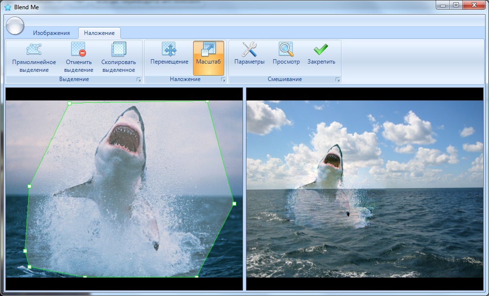
- Java program + source
- Photos taken with the program Blend Me
Source: https://habr.com/ru/post/213403/
All Articles