Home current measurement
There is a whole class of devices called Ethernet Relay that allow you to remotely control the connected load through the network. Most of them are quite expensive - closer to $ 100, and deliberately inferior in price and flexibility in setting up a bundle of, say, Raspberry Pi + PiFace . And what if the task is not only to turn on and off the load, but also to measure the current flowing? This requires the actual sensor (on the shunt or Hall effect) and the ADC (the Raspberry Pi does not contain an integrated ADC). As a sensor, you can take an inexpensive ACS712, and as an ADC, for example, ADC-Pi .
I didn’t like ADC-Pi for two reasons:
All Arduino already has an ADC (8-bit, but this is quite enough), sketches for Arduino are executed with the necessary stability, there are various options for communicating with Raspberry Pi, the simplest of which is a USB cable. And of course, an attractive price.
A bunch that I used is shown in the picture.

Measuring the current is a simple task, if not for one “but”: the physical sensors are “noisy”. The figure shows an example of the actual and calculated current values for my circuit with 512 consecutive measurements.

Thus, the task of measuring alternating current is to calculate the amplitude of a sinusoid from a set of actual measurements containing a significant proportion of errors.
')
Formula AC (who forgot - see wiki )
i = Im sin (ωt +)
Where:
Im is the maximum current value
ω - angular frequency
t - time (sequence number) changes
ψ - the initial phase of the current
You can try to find the necessary parameters using analytical tools. And here we are in for a pleasant surprise: last fall (2013), the Wolfram company released a version of its wonderful Mathematica package for the Raspberry Pi . Free (for home use). And we can apply it to analyze the data read from the sensor.
An example of calling a billing package in Raspberry Pi:
The calc_current.wl script itself is below with comments:
Read data from the file passed as parameter. The file contains lines of the form <measurement number>, <value>.
When the data is read, you can do a Fourier analysis (Fast Fourier Transform) in order to determine, approximately, the number of sinusoid cycles on the available sample. The dependence of the current strength on time is non-linear, and the approximate angular velocity calculated from the FFT and transmitted as the initial value will dramatically increase the chances of finding the correct sinusoid parameters.
If the maximum FFT value is not much different from the average for the sample, we can conclude that there is no pronounced sinusoid, all indicators are “noise”, and the real current is zero.
If a pronounced sinusoid is found, you can try to find the parameters of the function using the most pronounced cycle to calculate the initial value of the angular velocity.
Knowing the physical characteristics of the ADC (dimension 1024, base voltage 5V) and the sensor (in my version 0.185V / A), one can calculate the effective amperage:
The proposed method works in most cases. The number of measurements, when NonlinearModelFit could not correctly pick up the parameters of the sine wave, was about 5 percent. However, each measurement requires a lot of time - I have an average of 5 seconds - to launch the wolfram application. Therefore…
Since the frequency of the alternating current in the network is stable and amounts (in Russia) to 50 Hz, the angular velocity can be calculated in advance and, instead of nonlinear regression, a linear regression can be obtained. Indeed,

or

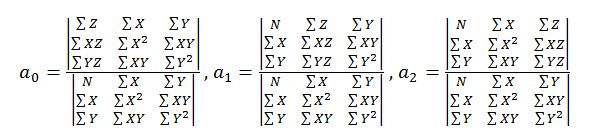
Differentiating with X and Y, we obtain a system of linear equations:

Solving the system according to Cramer, we obtain the values of the coefficients:
Then, according to the Pythagorean theorem, the maximum current value will be:

The Arduino sketch that implements this algorithm can be found on Github . The method provides good measurement accuracy: for the circuit in the figure, the measured current value was stably 0.13A, which corresponds to a consumption of 29.9 W at a voltage of 230V. The nominal value of the light bulb, which served as a load, is 30 watts.
By the way, for Arduino there are also shields with relays and all the functionality of control and load monitoring can be implemented on this platform. Raspberry Pi in this case will be used only for organizing a convenient user interface, for example, via a web server and as a sheduler.
I didn’t like ADC-Pi for two reasons:
- at the frequency of measurements that is required to determine the AC power in the network, this ADC gives a very large error (most likely I did not completely understand the registers)
- Using this ADC in conjunction with Raspberry Pi for Linux is difficult to ensure the necessary stability of the measurement period. Installing and configuring RTOS Linux only for this task seemed to me too complex, especially since there is a simpler and proven solution: Arduino
All Arduino already has an ADC (8-bit, but this is quite enough), sketches for Arduino are executed with the necessary stability, there are various options for communicating with Raspberry Pi, the simplest of which is a USB cable. And of course, an attractive price.
A bunch that I used is shown in the picture.
Measuring the current is a simple task, if not for one “but”: the physical sensors are “noisy”. The figure shows an example of the actual and calculated current values for my circuit with 512 consecutive measurements.
Thus, the task of measuring alternating current is to calculate the amplitude of a sinusoid from a set of actual measurements containing a significant proportion of errors.
')
Attempt number one
Formula AC (who forgot - see wiki )
i = Im sin (ωt +)
Where:
Im is the maximum current value
ω - angular frequency
t - time (sequence number) changes
ψ - the initial phase of the current
You can try to find the necessary parameters using analytical tools. And here we are in for a pleasant surprise: last fall (2013), the Wolfram company released a version of its wonderful Mathematica package for the Raspberry Pi . Free (for home use). And we can apply it to analyze the data read from the sensor.
An example of calling a billing package in Raspberry Pi:
pi@raspi ~ $ wolfram -script calc_current.wl datafile=/tmp/data.csvThe calc_current.wl script itself is below with comments:
Read data from the file passed as parameter. The file contains lines of the form <measurement number>, <value>.
data=Import[$CommandLine[[4]]]When the data is read, you can do a Fourier analysis (Fast Fourier Transform) in order to determine, approximately, the number of sinusoid cycles on the available sample. The dependence of the current strength on time is non-linear, and the approximate angular velocity calculated from the FFT and transmitted as the initial value will dramatically increase the chances of finding the correct sinusoid parameters.
fourier=Take[Abs[Fourier[data[[All,2]]]],{2,256}]If the maximum FFT value is not much different from the average for the sample, we can conclude that there is no pronounced sinusoid, all indicators are “noise”, and the real current is zero.
topcycle=Ordering[fourier,-1]avg=Mean[fourier]top=fourier[[topcycle[[1]]]]If[top < 10 * avg, Print["No AC"]; Exit[]]If a pronounced sinusoid is found, you can try to find the parameters of the function using the most pronounced cycle to calculate the initial value of the angular velocity.
nlm=NonlinearModelFit[data, a Sin[bx + c]+d, {a,{b, 2 Pi * topcycle[[1]] / 512}, c, d},x]Knowing the physical characteristics of the ADC (dimension 1024, base voltage 5V) and the sensor (in my version 0.185V / A), one can calculate the effective amperage:
imax=Abs[nlm["BestFitParameters"][[1]][[2]]] / (1024 / 5 * 0.185)Print["Imax=", imax]iefc=imax / Sqrt[2]Print["Iefc=", iefc]Print["Power=", iefc * 230]The proposed method works in most cases. The number of measurements, when NonlinearModelFit could not correctly pick up the parameters of the sine wave, was about 5 percent. However, each measurement requires a lot of time - I have an average of 5 seconds - to launch the wolfram application. Therefore…
Attempt number two
Since the frequency of the alternating current in the network is stable and amounts (in Russia) to 50 Hz, the angular velocity can be calculated in advance and, instead of nonlinear regression, a linear regression can be obtained. Indeed,

or

Differentiating with X and Y, we obtain a system of linear equations:

Solving the system according to Cramer, we obtain the values of the coefficients:

Then, according to the Pythagorean theorem, the maximum current value will be:

The Arduino sketch that implements this algorithm can be found on Github . The method provides good measurement accuracy: for the circuit in the figure, the measured current value was stably 0.13A, which corresponds to a consumption of 29.9 W at a voltage of 230V. The nominal value of the light bulb, which served as a load, is 30 watts.
By the way, for Arduino there are also shields with relays and all the functionality of control and load monitoring can be implemented on this platform. Raspberry Pi in this case will be used only for organizing a convenient user interface, for example, via a web server and as a sheduler.
Source: https://habr.com/ru/post/212459/
All Articles