Search for routes for 1 person-month
One day, our project required routing functionality. We do not have a lot of programmers, but rather the opposite, so we wanted to find some kind of ready-made solution, we searched and did not find anything good.
We had the road graph data, but in such a way that it is not so easy to submit them to any library or some middle-ware. And, frankly, we did not find the middle-ware for navigation, so that it was simply integrated into our system (thanks, if someone tells you where to look). Therefore, they decided to make their own, using the maximum existing libraries for everything.

')
On the process of developing the service and tell.
About the graph.
A few words about the data. We receive data from a third-party supplier; we cannot influence the format and composition of data. Road data is in the form of a ArcView (Shapefile) file. All streets are divided into segments from the intersection to the intersection, each segment attributes are associated:
- unique segment identifier
- geometric polyline depicting a road segment
- data on the allowed maximum speed of traffic rules
- data on the possibility of reversal at the beginning and end of the segment
- a sign of one-way traffic on the segment
- Z is the level of the beginning and end of the segment (for example, the entrance to the overpass has a level 0 at the beginning and a level 1 at the end)
In addition, there is a separate file with motion restrictions imposed by logic and / or traffic regulations. Each restriction is a vector of identifiers that refer to street segments (from the first file), the consecutive movement of which is prohibited.
An example of how it all looks, hangs in the title of the post (red - bans, unfortunately, our software in this case does not allow to draw bans with the direction).
For the algorithms to work on a graph, it is required that the graph be presented in some generally accepted form, for example, as a list of connectedness of vertices, or a connectedness matrix. That is, data on vertices and the connections between them are actually required. Since the vertex information in our data is very incomplete, there is only data about their geometric location, we had to process it so that all vertices get unique identifiers.
We took the geometric location of the vertices as a basis, but there was one circumstance: the coordinates of the final vertices of the segments did not always coincide by 100%, for example, at intersections (perhaps the defects of the work of GIS system operators, I don’t know exactly). Therefore, we decided to consider as one vertex of the graph all the end points of the segments having the same Z-level and separated from each other no further than 1 meter.
There are approximately 140,000 total road segments in our data, which means approximately 280,000 end points. Accordingly, we needed some kind of non-legged algorithm for finding all neighbors at a distance of up to 1 meter of each point. The frontal search of all pairs has a quadratic complexity and works excessively long. Since we decided that our program will work directly with the original data view, that is, with Shape-files (reasons: easy to update, no need to maintain, document, version your own storage format), we needed an efficient vertex identification algorithm.
They came up with this (hereinafter C ++ code):
1. Made a container for the edges of the graph:
Multimap, because we decided not to introduce new identifiers of segments / edges of the graph, but to keep information about the forward and reverse edges, respectively, with the same identifiers. It was probably not the right decision, because in my opinion it complicated the logic of some procedures, but in the beginning it seemed that it would be normal.
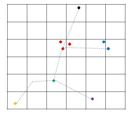
Figure 1.
2. The coordinate plane was divided into squares by a meter per meter (Figure 1).
Each vertex has a key mapped:
3. Made a hash container
When viewing the list of segments of the street network, we build a list of elements containing the identifiers of the initial and final vertices, the edge identifier, and related information, that is, in fact, a graph as a list of adjacent vertices.
We try to add the starting and ending point of the segment to SPHash according to the key calculated in paragraph 2. If there are already points with such a key in the container, then we do not add a new point, but return the identifier already existing (provided that the existing point in the container is at the same Z level as the one being added).
If there is nothing on the key in the container, then add a point to the container and return the identifier of the added point.
True points, the distance between which is less than 1 meter, may have different keys, so we check the container not only by the calculated key, but also by the 8 neighboring ones:
merge () builds a list of identifiers of the nearest points in the near vector.
Having received the list of identifiers of neighbors (in fact, candidates for merging into one vertex), we compare the points, calculating the exact Euclidean distance between them. And if it is less than the specified, then we assume that the points are the same and merge into one vertex (painted in one color in the figure), returning the identifier of the suitable vertex already in the cell with the key getKey (xPart, yPart).
At the start, this processing takes about 1 second, which suits us.
4. As a result, we obtain that neighboring points closer to a given threshold receive one identifier.
Now we have a list of adjacent vertices. The time complexity of obtaining such a list linearly depends on the number of vertices, because we process each one exactly 1 time, and the search and insertion operations in the hash container have asymptotically constant complexity.
As you should have already noticed, we do not process intermediate vertices of a broken street segment, since they do not affect the topology of the graph (in the middle of the segment, no maneuver can be made, in any case, we have no data about it).
If we would break the polyline into its constituent segments and consider each segment as an edge, then in the graph, instead of about 140,000 edges, there would already be about 600,000. The time to search for a path would increase significantly, at the end I will show this difference in absolute values.
Stayed the final touch. Restrictions, or prohibited maneuvers.
The restriction prohibits any maneuver, for example, turning left at an intersection. Initially, the data is a list of segments, the consecutive movement of which is prohibited.
I will give an example:
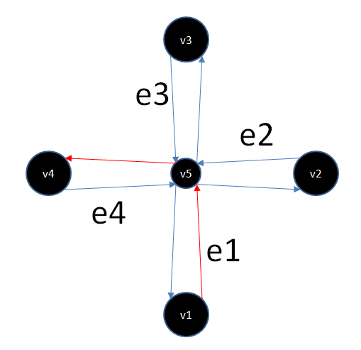
Fig. 2
Red arrows indicate a forbidden maneuver, numbers denote segment identifiers. In fact, in the data, this prohibition looks like {e1, e4}.
With such a view of the prohibitions, it is very difficult to work in the process of laying a route, so we decided to locally transform the graph so that the forbidden maneuver was impossible in the graph purely topologically, while all other allowed maneuvers remained possible.
To do this, we have duplicated the vertices that are included in the forbidden maneuver. And through these duplicated vertices, we fixed the ribs so as to create allowed maneuvers, and for the forbidden maneuver such a route simply does not create.
When cloning a vertex, its geometric location remains the same (the vertices v6 and v5 shown in the figure are actually geometrically in the same place and spaced apart in the figure for convenience), for the new vertex, of course, a new identifier is allocated.
I will illustrate with the example of the intersection with the forbidden left turn above:

Figure 3.
It can be seen that on the graph with the changed topology, it is no longer possible to make a left turn along the forbidden path at the intersection, while all the allowed maneuvers remained possible.
Restrictions from more than 2 edges are processed according to the same principle, but generate more new vertices and edges, these transformations affect the size of the graph, but not significantly (the growth of the number of edges by about 5%). In our data there are about 5000 restrictions from two segments and about 400 from three).
Here is an illustration of how a graph is transformed under the action of a 3-edge constraint:
It was:

Figure 4.
It became:

Figure 5.
It must be said that the implementation of the graph transformation algorithm became the most difficult stage of the whole work (it took about 30% of the time) and that was where the greatest number of bugs were. This is partly due to not very good development of the data storage structure. So if something remains unclear - it is not scary, it was really not easy, ask questions, try to answer.
About the tools.
And so now we had a graph presented in a convenient form with all the restrictions on which it was possible to lay routes. As an algorithm, we decided to try the classic Dijkstra algorithm, which is a good implementation in the boost library.
There is nothing special to add, for boost :: graph there is good documentation and even books, we took the code of one of the examples and used it with minor changes.
The next step was processing requests. We decided that it was convenient if the service could make a route with only the start and end point given by the coordinates. This means that we must quickly find the initial and final vertices in the graph, which are located as close as possible to the corresponding points of the query.
To do this, it was necessary to quickly be able to find the point closest to the user-defined point on the street network (the user may want a route from a point outside the road network).
It is appropriate to recall that the segments of the road-street network in our data are broken, so we had to find the closest point to the given point on the broken line (this could be the point lying on the broken line, or its initial or final vertex).
There are quite a few broken lines (140,000), but you need to search quickly. Search through all segments too slowly. Here a fresh version of the library boost :: geometry, where spatial indices (boost :: geometry :: index) appeared already with the support of such an object as a broken line (linestring), came to the rescue.
Using this index, we quickly find several closest candidates, of which then the exact segment that most closely passes near a given point is determined by an exact algorithm.
For reading SHP files, we used the GDAL library, for converting between geographic coordinate systems (we work in the local system of the city, historically), and it’s more convenient for the user to use GPS (WGS84) coordinates) they took the proj4 library, and for iconv text conversion tasks.
About the details.
- route to the middle of the edge
Let me remind you that our graph is a topological representation of the road network, the geometrical details for the operation of the Dijkstra algorithm are unimportant. But the geometric aspect is important to the user. Recall that the Dijkstra algorithm builds the shortest routes from a given vertex of the graph to all the others (including the desired final vertex).
So we must determine the initial vertex, but we search the index among the broken lines, that is, in fact, among the edges. How to understand from which vertex (in the graph) you need to make a route, because there are no intermediate segment peaks, which means that you need to select either the initial or the final vertex of the found segment.

Figure 6.
However, this solution will not be convenient for the user; imagine a long highway without turns and turns (and this often happens). The user will be very surprised to see how the route was built from the point located a kilometer from the one he set (because there was no closer to the next segment of the other peaks). This is bad. In addition, as shown in Figure 6 (red dotted lines), selecting the nearest vertex of the segment will sometimes mean a longer way to the goal, which is not good at all. So we had to somehow create the appearance of the fact that there are more peaks in our graph and they are located more often, but in such a way that it does not affect the running time of the pathfinding algorithm.
Several approaches were considered with their advantages and disadvantages:
1) two searches from the initial and final vertices of the segment and the choice of the path that is shorter, taking into account the distance from the user's point from the corresponding end of the segment.
plus: easy to implement
minus: double search for the shortest path with the corresponding slowdown time.
2) creating a redundant graph: all geometric vertices of the road network segments are transformed into graph vertices.
plus: easy to implement
minuses: a significant increase in the operating time of the Dijkstra algorithm, in some cases does not solve the problem (straight long stretch of road)
3) complement the graph with temporary vertices and edges at the time of the request and return the graph to its initial state after the route has been found.
plus: one search route, no need to inflate the graph, fast running.
minus: harder to implement than other methods
We have chosen the third way. A graph is temporarily added to the graph corresponding to the closest to the user point lying on the broken segment and 2 edges (corresponding to the segments of the segment to the starting and ending vertices, or just one of them, if the one-way segment) are added to the graph, a search is performed, after which the temporary vertices and edges are removed from the graph.
- output to the web
In fact, our program does not work with the network at all, it reads the standard input and writes the answer to the standard output, and the entire interface with the network and dispatching are done by a separate program on node.js.
- multithreading
It's simple. Our program works in 1 stream. But if you really need to load all the server cores, then you can run 1 instance for each kernel, the benefit is 1 process requires to store the graph, about 300 MB (and this size can be reduced by 2-3 times, but we haven’t set ourselves this task yet as unnecessary). How to distribute requests by processes? Since we have an external dispatcher, it can do the distribution of requests to running processes, as well as monitor their performance, etc.
Another way to load all cores: creating a multi-threaded program in C ++, seemed to us more difficult. First of all, it would be necessary to write the network code in C ++ (we almost all server-side of the project was written on node.js and we knew that it was much easier to work with the network on it), or to make a more complex interface to the external controller compared to stdin / stdout. Secondly, we don’t have a read-only graph because of temporary vertices and edges, which means we would have to very carefully synchronize the worker threads so that we don’t kill the performance on the one hand, and we don’t run into the corresponding problems of the multithreaded code on the other. found the advantages of this approach (at the moment) to do so.
In conclusion, a small statistic:
The whole program turned out to be only 1500 lines, plus a few dozen lines of the dispatcher on node.js, 1 person was coding in C ++, it took about 1 month + time and a couple of colleagues helped with the ideas and debugging. It seems to us quite well for such a not very elementary task.
The average time to search for a route (on Core i7 3.4 Ghz) is about 60-65 ms. By the way, I promised to tell the time of work on the graph, where each segment of the broken road segment turns into a separate edge of the graph, this is about 250 ms, a noticeable difference, you will agree.
Thank you for your attention to those who read to the end.
We had the road graph data, but in such a way that it is not so easy to submit them to any library or some middle-ware. And, frankly, we did not find the middle-ware for navigation, so that it was simply integrated into our system (thanks, if someone tells you where to look). Therefore, they decided to make their own, using the maximum existing libraries for everything.
')
On the process of developing the service and tell.
About the graph.
A few words about the data. We receive data from a third-party supplier; we cannot influence the format and composition of data. Road data is in the form of a ArcView (Shapefile) file. All streets are divided into segments from the intersection to the intersection, each segment attributes are associated:
- unique segment identifier
- geometric polyline depicting a road segment
- data on the allowed maximum speed of traffic rules
- data on the possibility of reversal at the beginning and end of the segment
- a sign of one-way traffic on the segment
- Z is the level of the beginning and end of the segment (for example, the entrance to the overpass has a level 0 at the beginning and a level 1 at the end)
In addition, there is a separate file with motion restrictions imposed by logic and / or traffic regulations. Each restriction is a vector of identifiers that refer to street segments (from the first file), the consecutive movement of which is prohibited.
An example of how it all looks, hangs in the title of the post (red - bans, unfortunately, our software in this case does not allow to draw bans with the direction).
For the algorithms to work on a graph, it is required that the graph be presented in some generally accepted form, for example, as a list of connectedness of vertices, or a connectedness matrix. That is, data on vertices and the connections between them are actually required. Since the vertex information in our data is very incomplete, there is only data about their geometric location, we had to process it so that all vertices get unique identifiers.
We took the geometric location of the vertices as a basis, but there was one circumstance: the coordinates of the final vertices of the segments did not always coincide by 100%, for example, at intersections (perhaps the defects of the work of GIS system operators, I don’t know exactly). Therefore, we decided to consider as one vertex of the graph all the end points of the segments having the same Z-level and separated from each other no further than 1 meter.
There are approximately 140,000 total road segments in our data, which means approximately 280,000 end points. Accordingly, we needed some kind of non-legged algorithm for finding all neighbors at a distance of up to 1 meter of each point. The frontal search of all pairs has a quadratic complexity and works excessively long. Since we decided that our program will work directly with the original data view, that is, with Shape-files (reasons: easy to update, no need to maintain, document, version your own storage format), we needed an efficient vertex identification algorithm.
They came up with this (hereinafter C ++ code):
1. Made a container for the edges of the graph:
typedef size_t EdgeID; typedef size_t VertexID; struct EdgeDesc { VertexID vtxSrc, vtxDest; EdgeInfo info; }; typedef std::unordered_multimap<EdgeID, EdgeDesc> EdgeMap; Multimap, because we decided not to introduce new identifiers of segments / edges of the graph, but to keep information about the forward and reverse edges, respectively, with the same identifiers. It was probably not the right decision, because in my opinion it complicated the logic of some procedures, but in the beginning it seemed that it would be normal.
Figure 1.
2. The coordinate plane was divided into squares by a meter per meter (Figure 1).
Each vertex has a key mapped:
static_assert(sizeof(size_t) >= 8, "size_t type should be 64 bit or larger"); auto keyPartX = [this](double x) { return (size_t)(x - bound_.first.x) + 1; }; auto keyPartY = [this](double y) { return (size_t)(y - bound_.first.y) + 1; }; auto getKey = [](size_t x, size_t y) { return x << (sizeof(size_t) / 2 * 8) | y; }; auto getKeyXY = [&keyPartX, &keyPartY, &getKey](double x, double y) { return getKey(keyPartX(x), keyPartY(y)); }; 3. Made a hash container
typedef size_t CellKey; typedef std::unordered_map<CellKey, std::vector<VertexID>> SPHash; When viewing the list of segments of the street network, we build a list of elements containing the identifiers of the initial and final vertices, the edge identifier, and related information, that is, in fact, a graph as a list of adjacent vertices.
We try to add the starting and ending point of the segment to SPHash according to the key calculated in paragraph 2. If there are already points with such a key in the container, then we do not add a new point, but return the identifier already existing (provided that the existing point in the container is at the same Z level as the one being added).
If there is nothing on the key in the container, then add a point to the container and return the identifier of the added point.
True points, the distance between which is less than 1 meter, may have different keys, so we check the container not only by the calculated key, but also by the 8 neighboring ones:
std::vector<size_t> near; size_t xPart = keyPartX(px); size_t yPart = keyPartY(py); near.clear(); merge(near, getKey(xPart, yPart)); merge(near, getKey(xPart + 1, yPart)); merge(near, getKey(xPart - 1, yPart)); merge(near, getKey(xPart, yPart + 1)); merge(near, getKey(xPart, yPart - 1)); merge(near, getKey(xPart + 1, yPart + 1)); merge(near, getKey(xPart + 1, yPart - 1)); merge(near, getKey(xPart - 1, yPart + 1)); merge(near, getKey(xPart - 1, yPart - 1)); merge () builds a list of identifiers of the nearest points in the near vector.
Having received the list of identifiers of neighbors (in fact, candidates for merging into one vertex), we compare the points, calculating the exact Euclidean distance between them. And if it is less than the specified, then we assume that the points are the same and merge into one vertex (painted in one color in the figure), returning the identifier of the suitable vertex already in the cell with the key getKey (xPart, yPart).
At the start, this processing takes about 1 second, which suits us.
4. As a result, we obtain that neighboring points closer to a given threshold receive one identifier.
Now we have a list of adjacent vertices. The time complexity of obtaining such a list linearly depends on the number of vertices, because we process each one exactly 1 time, and the search and insertion operations in the hash container have asymptotically constant complexity.
As you should have already noticed, we do not process intermediate vertices of a broken street segment, since they do not affect the topology of the graph (in the middle of the segment, no maneuver can be made, in any case, we have no data about it).
If we would break the polyline into its constituent segments and consider each segment as an edge, then in the graph, instead of about 140,000 edges, there would already be about 600,000. The time to search for a path would increase significantly, at the end I will show this difference in absolute values.
Stayed the final touch. Restrictions, or prohibited maneuvers.
The restriction prohibits any maneuver, for example, turning left at an intersection. Initially, the data is a list of segments, the consecutive movement of which is prohibited.
I will give an example:

Fig. 2
Red arrows indicate a forbidden maneuver, numbers denote segment identifiers. In fact, in the data, this prohibition looks like {e1, e4}.
With such a view of the prohibitions, it is very difficult to work in the process of laying a route, so we decided to locally transform the graph so that the forbidden maneuver was impossible in the graph purely topologically, while all other allowed maneuvers remained possible.
To do this, we have duplicated the vertices that are included in the forbidden maneuver. And through these duplicated vertices, we fixed the ribs so as to create allowed maneuvers, and for the forbidden maneuver such a route simply does not create.
When cloning a vertex, its geometric location remains the same (the vertices v6 and v5 shown in the figure are actually geometrically in the same place and spaced apart in the figure for convenience), for the new vertex, of course, a new identifier is allocated.
I will illustrate with the example of the intersection with the forbidden left turn above:

Figure 3.
It can be seen that on the graph with the changed topology, it is no longer possible to make a left turn along the forbidden path at the intersection, while all the allowed maneuvers remained possible.
Restrictions from more than 2 edges are processed according to the same principle, but generate more new vertices and edges, these transformations affect the size of the graph, but not significantly (the growth of the number of edges by about 5%). In our data there are about 5000 restrictions from two segments and about 400 from three).
Here is an illustration of how a graph is transformed under the action of a 3-edge constraint:
It was:

Figure 4.
It became:

Figure 5.
It must be said that the implementation of the graph transformation algorithm became the most difficult stage of the whole work (it took about 30% of the time) and that was where the greatest number of bugs were. This is partly due to not very good development of the data storage structure. So if something remains unclear - it is not scary, it was really not easy, ask questions, try to answer.
About the tools.
And so now we had a graph presented in a convenient form with all the restrictions on which it was possible to lay routes. As an algorithm, we decided to try the classic Dijkstra algorithm, which is a good implementation in the boost library.
There is nothing special to add, for boost :: graph there is good documentation and even books, we took the code of one of the examples and used it with minor changes.
The next step was processing requests. We decided that it was convenient if the service could make a route with only the start and end point given by the coordinates. This means that we must quickly find the initial and final vertices in the graph, which are located as close as possible to the corresponding points of the query.
To do this, it was necessary to quickly be able to find the point closest to the user-defined point on the street network (the user may want a route from a point outside the road network).
It is appropriate to recall that the segments of the road-street network in our data are broken, so we had to find the closest point to the given point on the broken line (this could be the point lying on the broken line, or its initial or final vertex).
There are quite a few broken lines (140,000), but you need to search quickly. Search through all segments too slowly. Here a fresh version of the library boost :: geometry, where spatial indices (boost :: geometry :: index) appeared already with the support of such an object as a broken line (linestring), came to the rescue.
Using this index, we quickly find several closest candidates, of which then the exact segment that most closely passes near a given point is determined by an exact algorithm.
For reading SHP files, we used the GDAL library, for converting between geographic coordinate systems (we work in the local system of the city, historically), and it’s more convenient for the user to use GPS (WGS84) coordinates) they took the proj4 library, and for iconv text conversion tasks.
About the details.
- route to the middle of the edge
Let me remind you that our graph is a topological representation of the road network, the geometrical details for the operation of the Dijkstra algorithm are unimportant. But the geometric aspect is important to the user. Recall that the Dijkstra algorithm builds the shortest routes from a given vertex of the graph to all the others (including the desired final vertex).
So we must determine the initial vertex, but we search the index among the broken lines, that is, in fact, among the edges. How to understand from which vertex (in the graph) you need to make a route, because there are no intermediate segment peaks, which means that you need to select either the initial or the final vertex of the found segment.

Figure 6.
However, this solution will not be convenient for the user; imagine a long highway without turns and turns (and this often happens). The user will be very surprised to see how the route was built from the point located a kilometer from the one he set (because there was no closer to the next segment of the other peaks). This is bad. In addition, as shown in Figure 6 (red dotted lines), selecting the nearest vertex of the segment will sometimes mean a longer way to the goal, which is not good at all. So we had to somehow create the appearance of the fact that there are more peaks in our graph and they are located more often, but in such a way that it does not affect the running time of the pathfinding algorithm.
Several approaches were considered with their advantages and disadvantages:
1) two searches from the initial and final vertices of the segment and the choice of the path that is shorter, taking into account the distance from the user's point from the corresponding end of the segment.
plus: easy to implement
minus: double search for the shortest path with the corresponding slowdown time.
2) creating a redundant graph: all geometric vertices of the road network segments are transformed into graph vertices.
plus: easy to implement
minuses: a significant increase in the operating time of the Dijkstra algorithm, in some cases does not solve the problem (straight long stretch of road)
3) complement the graph with temporary vertices and edges at the time of the request and return the graph to its initial state after the route has been found.
plus: one search route, no need to inflate the graph, fast running.
minus: harder to implement than other methods
We have chosen the third way. A graph is temporarily added to the graph corresponding to the closest to the user point lying on the broken segment and 2 edges (corresponding to the segments of the segment to the starting and ending vertices, or just one of them, if the one-way segment) are added to the graph, a search is performed, after which the temporary vertices and edges are removed from the graph.
- output to the web
In fact, our program does not work with the network at all, it reads the standard input and writes the answer to the standard output, and the entire interface with the network and dispatching are done by a separate program on node.js.
- multithreading
It's simple. Our program works in 1 stream. But if you really need to load all the server cores, then you can run 1 instance for each kernel, the benefit is 1 process requires to store the graph, about 300 MB (and this size can be reduced by 2-3 times, but we haven’t set ourselves this task yet as unnecessary). How to distribute requests by processes? Since we have an external dispatcher, it can do the distribution of requests to running processes, as well as monitor their performance, etc.
Another way to load all cores: creating a multi-threaded program in C ++, seemed to us more difficult. First of all, it would be necessary to write the network code in C ++ (we almost all server-side of the project was written on node.js and we knew that it was much easier to work with the network on it), or to make a more complex interface to the external controller compared to stdin / stdout. Secondly, we don’t have a read-only graph because of temporary vertices and edges, which means we would have to very carefully synchronize the worker threads so that we don’t kill the performance on the one hand, and we don’t run into the corresponding problems of the multithreaded code on the other. found the advantages of this approach (at the moment) to do so.
In conclusion, a small statistic:
The whole program turned out to be only 1500 lines, plus a few dozen lines of the dispatcher on node.js, 1 person was coding in C ++, it took about 1 month + time and a couple of colleagues helped with the ideas and debugging. It seems to us quite well for such a not very elementary task.
The average time to search for a route (on Core i7 3.4 Ghz) is about 60-65 ms. By the way, I promised to tell the time of work on the graph, where each segment of the broken road segment turns into a separate edge of the graph, this is about 250 ms, a noticeable difference, you will agree.
Thank you for your attention to those who read to the end.
Source: https://habr.com/ru/post/211388/
All Articles