How I invent a method of simulating annealing

Good time, Habr!

I was inspired to write this paper reading “Introduction to optimization. Imitation annealing . It so happened that just recently I ran into the task of a traveling salesman, and to solve it I came up with an algorithm, the essence of which, as it turned out, is very close to the idea of ​​the annealing simulation algorithm described in this article. Moreover, there is even a “reference” to my idea, and similar discussions were held in the comments, so I decided that it would be interesting for the community to look at the implementation.

I'll start with a little intro. I am a student of the 1st year of the master's program in the specialty "Software Engineering", and this semester we had a course of distributed systems, in which I got the task of a traveling salesman. And it would be okay, but with the requirement to implement it in parallel and using four different technologies (Windows Azure, openmpi library, Go programming language, Limbo programming language in OS Inferno). If I came across such a qualitatively described solution, the problems would be much less, but at that time I was able to find out only the branch and bound method. Vile thing must be said, because the idea to implement it in parallel, and besides using technologies previously unknown, seemed to me at once unsuccessful. As a result of much deliberation of this problem, I came to an algorithm that turned out to be surprisingly simple, although not very effective. Nevertheless, I managed to pass it on to the teacher, and the “research” work on the algorithm, as it turned out, would be quite suitable for this article. Unless for article I will give the program code on pure C # and without use of parallel troubles.
I will not dwell on the issues of what is optimization and annealing method, I think that in the article “Introduction to optimization. Annealing imitation » it is explained just fine, and for those who wish to understand more, I advise you to read it. I will go straight to the description of the traveling salesman problem and my solution.

Task analysis

The traveling salesman problem is one of the most well-known combinatorial optimization problems, which consists in finding the most profitable route that passes through the specified cities once and then returns to the source city. In terms of the problem, the route profitability criterion is indicated (shortest, cheapest, aggregate criterion, etc.).
If we formalize the task, then we are talking about a kind of weighted graph (for simplicity, for the sake of discussion, we set it undirected, although in the general case this may not be so), in which we need to find a circumvention path that passes through all the vertices exactly once and returns to the starting point, at the same time the minimum weight (for further reasoning I will call the vertices of the graph cities, and the weight of the edge - the distance between cities).
')


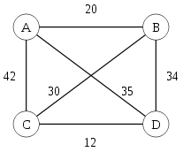
Such a graph can be represented as a symmetric matrix with zeros on the main diagonal (the length of the path from the city to itself is zero).

Algorithm of the decision

In this part I will describe both ways of implementing the algorithm (sequential and parallel), and give the program code for the sequential version.

Sequential implementation
Create an arbitrary starting path containing all the vertices once and returning to the starting position. Then we randomly swap two cities and compare the lengths of the old and the new ways. If the new path is shorter, save it. If not, then we increase the counter. When the counter takes a predetermined value, stop the algorithm, the last path found in this way will be considered the best.

Parallel implementation
Create an arbitrary initial path containing all the vertices once and returning to the initial position and “distribute” it to each of the parallel processes / threads. Each of them, independently of each other, performs the described operations to find the optimal path and returns the result found. The main stream, if implied, chooses the best from the results obtained.

As you can see, the idea is very simple. What is great, it is also very easy to implement that in the serial, in the parallel version, since in the second case, there is no struggle for shared resources and there is no exchange of information between the threads themselves, which simplifies programming unimaginably.

C # software implementation

class CCities { //   public Point[] Coordinate; public CCities(int N, int maxValue) //maxValue -   pictureBox   { Random random = new Random(); Coordinate = new Point[N]; //   ,   pictureBox,        //     int minBorder = (int)(maxValue * 0.05); int maxBorder = (int)(maxValue * 0.95); for (int i = 0; i < N; i++) { Coordinate[i] = new Point(random.Next(minBorder, maxBorder), random.Next(minBorder, maxBorder)); } } } 

  class CPath { //   double[,] distance; //     public int[] Path; public CPath(CCities map) { //      distance = new double[map.Coordinate.Length, map.Coordinate.Length]; //  ,        for (int j = 0; j < map.Coordinate.Length; j++) { distance[j, j] = 0; for (int i = 0; i < map.Coordinate.Length; i++) { double value = Math.Sqrt(Math.Pow(map.Coordinate[i].X - map.Coordinate[j].X, 2) + Math.Pow(map.Coordinate[i].Y - map.Coordinate[j].Y, 2)); distance[i, j] = distance[j, i] = value; } } //   //  1  - ,       0 -      ""  Path = new int[map.Coordinate.Length + 1]; for (int i = 0; i < map.Coordinate.Length; i++) { Path[i] = i; } Path[map.Coordinate.Length] = 0; } //,      public void FindBestPath() { Random random = new Random(); for (int fails = 0, F = Path.Length * Path.Length; fails < F; ) { //    //      int p1 = 0, p2 = 0; while (p1 == p2) { p1 = random.Next(1, Path.Length - 1); p2 = random.Next(1, Path.Length - 1); } //  double sum1 = distance[Path[p1 - 1], Path[p1]] + distance[Path[p1], Path[p1 + 1]] + distance[Path[p2 - 1], Path[p2]] + distance[Path[p2], Path[p2 + 1]]; double sum2 = distance[Path[p1 - 1], Path[p2]] + distance[Path[p2], Path[p1 + 1]] + distance[Path[p2 - 1], Path[p1]] + distance[Path[p1], Path[p2 + 1]]; if (sum2 < sum1) { int temp = Path[p1]; Path[p1] = Path[p2]; Path[p2] = temp; } else { fails++; } } } //   public double PathLength() { double pathSum = 0; for (int i = 0; i < Path.Length - 1; i++) { pathSum += distance[Path[i], Path[i + 1]]; } return pathSum; } } 

Examples of the algorithm

Algorithm health analysis

Let me prove first the parallelization efficiency of such an algorithm. Since each of the parallel processes starts working with the same initial conditions, the probability of finding the optimal solution for each of them will be the same. Take it for p . Then the probability of not finding such a solution is q = 1 - p . Thus, the probability P that at least one of the processes will find the optimal path is equal to:


where K is the number of processes running in parallel. Such a dependence very quickly tends to 1 even for small p . The figure shows a plot of P (K) for p = 0.1 (the “de jure” schedule should be discrete, but I hope you will forgive me such a liberty):



It can be seen that already at K = 6..7 the probability P becomes equal to 0.5. That is, the benefits of using multiple processes are obvious - a very rapid increase in probability.
We now find the probability p for one process. Obviously, it is inversely proportional to the size of the N matrix and is directly proportional to the value of F , which the counter reaches when the algorithm stops its work. A more accurate estimate, unfortunately, is almost impossible to give. Almost the only thing we can say about the graph is that the number of different paths is equal to (N-1)! ⁄2 (subtract one because one city is the starting one and obviously does not participate in the search, but we divide by two because that the same path can be walked in both directions).
Thus, it is possible to estimate the desired probability only experimentally. A series of experiments was carried out for different parameters of N. The limit for the counter is F = N ^ 2 . For each N , 10,000 runs were performed and the results are listed in the table:



Let me explain the notation:
P (min) is the probability to find the optimal solution. P (X%) is the probability to find a solution that differs from the optimal one by no more than X% . That is, for example, for P (10%), such solutions will be those that fall in the interval [min, min + (max-min) * 0.1] , where min and max are the minimum and maximum respectively found paths.
There should be a digression and say this. Of course, such an analysis does not claim any real accuracy, since even 10,000 experiments are very few for obtaining the desired regularities (when restarting, the result may be completely different), and, most importantly, there is no guarantee that the algorithm has found best possible path. For evaluation, he operates with knowledge of the best of those found, but far from the fact that he is also the best of all. Nevertheless, I think it is possible to use the results obtained, if not for quantitative, but at least for a qualitative understanding of the operation of the algorithm.
We illustrate the same results:



Advantages of the method

• "Ideological" simplicity of the algorithm;
• Ease of implementation in both sequential and parallel versions;
• The rapidly growing efficiency of the algorithm with its parallel implementation;
• High probability of finding a solution that is close to optimal.

Disadvantages of the method

• Very quickly, the falling probability of finding the exact solution with increasing N;
• The difficulty of accurately estimating the probability of finding a solution;
• The lack of interconnection between threads in a parallel version leads to the fact that each of the threads can find the same bad solutions and not optimize the overall result (with very bad luck, all threads can just do the same work up to each iteration and return one and the same the same way in the end. It is very unlikely, but it is possible).

Algorithm optimization
In the process of work and research method, I suggested the following possible ways to improve the algorithm:

• Adding "history" already proven paths. At the moment, the algorithm does not remember the tested paths and does not control the new variants obtained at each iteration. Adding the function of checking and screening out such paths should greatly affect the accuracy of the result;
• Perhaps there is a way to more "fine" setting the control value of the counter. As can be seen from the test graphs, with the current settings ( F = N ^ 2 ), a “hole” appears in the area of N = 20 matrixes. I do not have an accurate understanding of the reasons for this behavior of the graph, but there is probably a way to select this value in a better way. .

Conclusion

I will be frank - it works so-so. I showed all the graphics and other results; you can see that the result of the work leaves much to be desired. In any case, this algorithm cannot be used to find the exact solution at this stage. On the other hand, he still finds more or less sane options, does not slip into frank lazy. If the task does not require an exact solution, and it comes down close to optimal, then this algorithm is quite efficient. Alternatively, you can use this algorithm to initially approximate the optimal value, and then run something like a search for options.
If you have any ideas for improving the performance of the algorithm, I will be very happy to hear them out.
I am also ready to listen to any constructive criticism of the article itself (design, presentation style, etc.).

For those who want to dig into the codes themselves, they uploaded an archive of the project to the mail cloud (written in VS2012, the project will be incompatible with earlier versions of VS; you will need .net framework 4.5 to run the program, the .exe file is located in the \ Salesman \ Salesman \ bin \ folder Debug)