Method of comparing algorithms and for what it may still be useful
Having recently read the article “Introduction to optimization. Annealing Simulation ” wanted to take part in the comparison of optimization algorithms. But after all it would be really good to compare them. And in the materials of the original article does not provide any quantitative data. So, I thought, we must first formulate the criteria for comparison. What I propose to do in this article.

So, by what criteria can you compare algorithms similar to "simulated annealing"? Most often compared:
• efficiency
• work speed
• memory usage
And I would like to add
• repeatability (i.e. check how stable the algorithm is in the results obtained).
As the first criterion we will use the length of the resulting route. I have no idea what is the best route on a randomly generated set of points. What to do? Let's try, for simplicity, to drive everything on one set. More pedantic, for greater reliability of the results, can then be expanded into several sets and average the results. In the meantime, you need to add the reading of the test set from the file so that the experiment can be repeated.
To determine the speed of work, we calculate the time spent by the processor on the algorithm, the benefit is in Octave such a function. Of course, on different computers, the result will also be different. Therefore, for comparison, all the results can be scaled by any one algorithm, always run. For example, according to the algorithm from the original article, since he was the first to fall.
At the expense of memory outright nothing was invented. Therefore, try to estimate on the fingers. As I understand it, the author’s main expenses are two indices arrays. One for the current route, the other for the candidate route. And, of course, an array of route points with two coordinates per point. The remaining costs will not be taken into account, since they will be different in different execution environments and do not depend on the size of the test data. (Perhaps here I am somewhat harsh, but quite open to suggestions). Total major expenses N * 4, where N - the number of points that need to be circumvented.
')
A small digression: everything described here was tested not in MatLab, as in the original article, but in Octave [http://www.gnu.org/software/octave/]. There are several reasons for this - firstly, I have it, secondly, its programming language is almost completely compatible with MatLab, and finally, it can be for everyone because it is free and publicly available.
To begin with, we are convinced of the compatibility for the existing code (it is downloaded by the link at the end of the original article). Everything works, but it turns out that there is no code generating the beautiful graphics presented in it. It does not matter - we will write our function from which we call the original algorithm and draw the result. Anyway, it will be needed for the entire body kit collection of statistics.
So the Analyze function:
The function for generating a file with an array of city coordinates did not begin to write. This can be done directly from the command line:
Yes, if someone noticed that the evaluation does not use the CalculateEnergy function from the original algorithm, then there are two reasons for this. Firstly, there is an idea to try working on other metrics, and the result is better to evaluate the Euclidean distance. And secondly, although the author of the original article described in detail the calculation of the Euclidean distance, the code in the sources calculates the Manhattan distance. Euclidean for two points is correctly calculated as follows:
Well, to determine how stable the result is from time to time, we will run it all in a cycle many times, collect the results and evaluate their average and the degree of scatter of the results:
The first disappointment is how long it all is! On the core i5-3450 3.1GHz 8Gb RAM computer, one pass runs an average of 578 seconds. So, for greater certainty, we wanted to start and average 1000 cycles, but this is ... 6.69 days. We had to run for 100 cycles and after about 16 hours 4 minutes (that is, the next morning) we have the result:
the average calculation time is 578.1926 (standard deviation in the sample is 3.056), the average length of the resulting path is 91.0844 (standard deviation is 2.49). That is, everything is more than stable, and, therefore, suitable for use. But how long. I could not resist and was tempted to do optimization.
The first candidate to speed up is distance estimation. Octave, like MatLab, is optimized for matrix computing - we will rewrite it for this. The function will take two arrays: A - the beginning of the segments, B - their ends, respectively:
To call this function, we will enter another one that will prepare the data by cyclically shifting the original array of points to obtain an array of the ends of the segments:
And, of course, you need to rewrite the function SimulatedAnnealing and GenerateStateCandidate to work directly with arrays of points. I will not give the full code, at the end there will be a link to the archive with all the sources for those who are interested.
We start, we look ... the average calculation time is 70.554 (standard deviation in the sample is 0.096), the average length of the resulting path is 90.403 (standard deviation 2.204).
The speed increase is more than eight times! It is no longer interesting to try further - such an increase will not be obtained. True, the memory consumption (according to the proposed method) is now two arrays of points in two coordinates (the current decision and the new candidate), that is ... N * 4. Nothing changed.
But, once we evaluate the algorithm, check the temperature data. The initial “energy” of the generated arrays of points fluctuates around 500 to 700 final routes at the output fluctuate around 90 plus / minus 5. Consequently, the temperatures chosen by the author practically only provide a limit of 100,000 iterations (by the way, it is also tightly clogged in the code. To prevent looping, I guess I raised up to ten million, why should I restrain myself when checking the algorithm?). And really, experimenting a little, we get about the same results for Tmax = 300 and Tmin = 0.001. At the same time, the execution time was reduced to 21 seconds.
Now we will try to compare with something. Initially, the idea was to compare with the Manhattan metric, but it turned out that it was implemented. Then this optimization. In short, we add code for the matrix calculation of the Manhattan distance and try for it. As interesting as another function of temperature change will show itself. Those who have been deceived by the linearity of the function of temperature change promised in the original article have to be disappointed - it is not. To understand this, just look at her schedule:
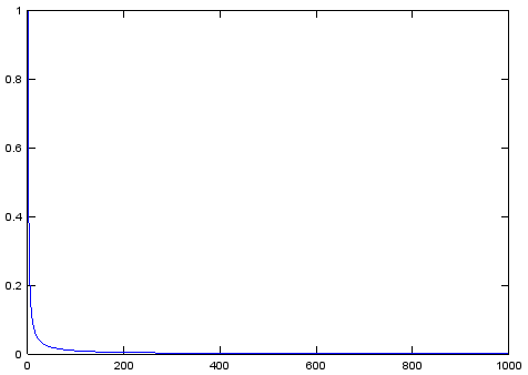
Probably there was a view of the linearity of the denominator of the function, because the denominators of all the other options used in science really look worse.
For comparison, let's try another temperature function T = Tmax * (A ^ k) where A is chosen, usually within 0.7 - 0.999. (When implemented, it is not greedy at all - Ti = A * Ti-1). Options for "annealing" with its use are called "quenching." It drops much faster to the minimum temperature, but flatter at the initial stage. That is, with it the algorithm experiments more at the beginning, but finishes work faster. So - a summary table of results:
Promised sources can be found at the link
Well, if you like it, you can compare it with something else after a while.
So, by what criteria can you compare algorithms similar to "simulated annealing"? Most often compared:
• efficiency
• work speed
• memory usage
And I would like to add
• repeatability (i.e. check how stable the algorithm is in the results obtained).
Criteria for evaluation
As the first criterion we will use the length of the resulting route. I have no idea what is the best route on a randomly generated set of points. What to do? Let's try, for simplicity, to drive everything on one set. More pedantic, for greater reliability of the results, can then be expanded into several sets and average the results. In the meantime, you need to add the reading of the test set from the file so that the experiment can be repeated.
To determine the speed of work, we calculate the time spent by the processor on the algorithm, the benefit is in Octave such a function. Of course, on different computers, the result will also be different. Therefore, for comparison, all the results can be scaled by any one algorithm, always run. For example, according to the algorithm from the original article, since he was the first to fall.
At the expense of memory outright nothing was invented. Therefore, try to estimate on the fingers. As I understand it, the author’s main expenses are two indices arrays. One for the current route, the other for the candidate route. And, of course, an array of route points with two coordinates per point. The remaining costs will not be taken into account, since they will be different in different execution environments and do not depend on the size of the test data. (Perhaps here I am somewhat harsh, but quite open to suggestions). Total major expenses N * 4, where N - the number of points that need to be circumvented.
')
A small digression: everything described here was tested not in MatLab, as in the original article, but in Octave [http://www.gnu.org/software/octave/]. There are several reasons for this - firstly, I have it, secondly, its programming language is almost completely compatible with MatLab, and finally, it can be for everyone because it is free and publicly available.
Analyzing ...
To begin with, we are convinced of the compatibility for the existing code (it is downloaded by the link at the end of the original article). Everything works, but it turns out that there is no code generating the beautiful graphics presented in it. It does not matter - we will write our function from which we call the original algorithm and draw the result. Anyway, it will be needed for the entire body kit collection of statistics.
So the Analyze function:
function [timeUsed, distTotal] = Analyze( ) % load points_data.dat cities % timeStart = cputime(); % result = SimulatedAnnealing(cities, 10, 0.00001); % timeUsed = cputime - timeStart; % distTotal = PathLengthMat(result); % plot(result(:,1), result(:,2), '-*'); drawnow (); end The function for generating a file with an array of city coordinates did not begin to write. This can be done directly from the command line:
cities = rand(100, 2)*10; save points_data.dat cities; Yes, if someone noticed that the evaluation does not use the CalculateEnergy function from the original algorithm, then there are two reasons for this. Firstly, there is an idea to try working on other metrics, and the result is better to evaluate the Euclidean distance. And secondly, although the author of the original article described in detail the calculation of the Euclidean distance, the code in the sources calculates the Manhattan distance. Euclidean for two points is correctly calculated as follows:
function [dist] = distEuclid(A, B) dist = (A - B).^2; dist = sum(dist); dist = sqrt(dist); end Well, to determine how stable the result is from time to time, we will run it all in a cycle many times, collect the results and evaluate their average and the degree of scatter of the results:
function [] = Statistics testNum = 1000; % timeUsed = zeros(testNum,1); distTotal = zeros(testNum,1); for n=1:testNum [timeUsed(n), distTotal(n)] = Analyze; end % time = [mean(timeUsed), std(timeUsed)] dist = [mean(distTotal), std(distTotal)] end The first disappointment is how long it all is! On the core i5-3450 3.1GHz 8Gb RAM computer, one pass runs an average of 578 seconds. So, for greater certainty, we wanted to start and average 1000 cycles, but this is ... 6.69 days. We had to run for 100 cycles and after about 16 hours 4 minutes (that is, the next morning) we have the result:
the average calculation time is 578.1926 (standard deviation in the sample is 3.056), the average length of the resulting path is 91.0844 (standard deviation is 2.49). That is, everything is more than stable, and, therefore, suitable for use. But how long. I could not resist and was tempted to do optimization.
Optimization
The first candidate to speed up is distance estimation. Octave, like MatLab, is optimized for matrix computing - we will rewrite it for this. The function will take two arrays: A - the beginning of the segments, B - their ends, respectively:
function [dist] = distEuclid(A, B) dist = (A - B).^2; dist = sum(dist, 2); dist = sqrt(dist); dist = sum(dist); end To call this function, we will enter another one that will prepare the data by cyclically shifting the original array of points to obtain an array of the ends of the segments:
function [length] = PathLengthMat(cities) citiesShifted = circshift(cities, 1); length = distEuclid(cities, citiesShifted); end And, of course, you need to rewrite the function SimulatedAnnealing and GenerateStateCandidate to work directly with arrays of points. I will not give the full code, at the end there will be a link to the archive with all the sources for those who are interested.
We start, we look ... the average calculation time is 70.554 (standard deviation in the sample is 0.096), the average length of the resulting path is 90.403 (standard deviation 2.204).
The speed increase is more than eight times! It is no longer interesting to try further - such an increase will not be obtained. True, the memory consumption (according to the proposed method) is now two arrays of points in two coordinates (the current decision and the new candidate), that is ... N * 4. Nothing changed.
But, once we evaluate the algorithm, check the temperature data. The initial “energy” of the generated arrays of points fluctuates around 500 to 700 final routes at the output fluctuate around 90 plus / minus 5. Consequently, the temperatures chosen by the author practically only provide a limit of 100,000 iterations (by the way, it is also tightly clogged in the code. To prevent looping, I guess I raised up to ten million, why should I restrain myself when checking the algorithm?). And really, experimenting a little, we get about the same results for Tmax = 300 and Tmin = 0.001. At the same time, the execution time was reduced to 21 seconds.
Exploring options
Now we will try to compare with something. Initially, the idea was to compare with the Manhattan metric, but it turned out that it was implemented. Then this optimization. In short, we add code for the matrix calculation of the Manhattan distance and try for it. As interesting as another function of temperature change will show itself. Those who have been deceived by the linearity of the function of temperature change promised in the original article have to be disappointed - it is not. To understand this, just look at her schedule:
Probably there was a view of the linearity of the denominator of the function, because the denominators of all the other options used in science really look worse.
For comparison, let's try another temperature function T = Tmax * (A ^ k) where A is chosen, usually within 0.7 - 0.999. (When implemented, it is not greedy at all - Ti = A * Ti-1). Options for "annealing" with its use are called "quenching." It drops much faster to the minimum temperature, but flatter at the initial stage. That is, with it the algorithm experiments more at the beginning, but finishes work faster. So - a summary table of results:
| Algorithm | Length (Scatter) | Time (scatter) | Memory |
|---|---|---|---|
| From the article | 91.0844 (2.4900) | 578.1926 (3.0560) | N * 4 |
| Matrix (10-0.00001) | 90.4037 (2.2038) | 70.554593 (0.096166) | N * 4 |
| Matrix (300-0.001) | 90.7956 (2.1967) | 20.94024 (0.16235) | N * 4 |
| Manhattan Matrix (10-0.00001) | 90.0506 (3.2397) | 70.96909 (0.7807) | N * 4 |
| Matrix "quenching" (300-0.001) | 92.0963 (2.3129) | 22.59591 (0.39581) | N * 4 |
Findings.
- The ability to quantify the results of the algorithm is useful even if there is no one to compare it with.
- If you take into account the features of the tool when writing a program - you can save a lot of time.
- If you choose the parameters for a specific task - you can save some more.
- It is pointless to compare algorithms for speed without optimization - the execution time will be almost a random variable.
- For modern processors, it is almost as easy to raise to the power and extract the root as it is to take a module - you can not be distorted and write math almost without simplifications.
- Many variations of one algorithm give very close results, if not a graphomaniac - use what is more convenient (or more familiar).
Promised sources can be found at the link
Well, if you like it, you can compare it with something else after a while.
Source: https://habr.com/ru/post/210812/
All Articles