Processing of digital images in remote sensing (remote sensing of the earth)
On Habré there were many articles about the use of various methods of image processing, including data classification, filtering. Many of these approaches are also used in remote sensing when processing digital images of the Earth.
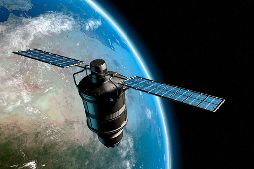
From the moment a snapshot is taken from a satellite, to being able to analyze it, it must go through a whole cycle of procedures to bring it into a form convenient for receiving and subsequent analysis of visual information.
Those who are interested in the process itself, please under the cat (traffic):
Before turning to the very essence, I would like to immediately introduce a number ofelementary concepts, which, surely, are already familiar to many, but, nevertheless, we will not deviate from reality. Those who are confident in their competence on this issue, let them go straight to the most interesting.
As everyone knows, a digital image is a matrix of pixels, the value of each of which is obtained by averaging over four components: the coordinates of space (x and y), wavelength and time.
The process of compiling the matrix itself goes this way: the solar radiation is reflected from the objects of the survey, the energy that falls on the sensor surface is fixed by it, then integrated, from which the integral pixel value is set. The integer value is obtained after converting the integral value into an electrical signal. Each pixel stores information in binary form. The more bits (memory) is allocated per pixel, the greater the number of values corresponding to one pixel, the more accurately the original discrete signal is approximated, and the more information a picture can store.
In CCD scanners, the already mentioned detectors scan the Earth and divide a continuous stream of data into pixels.
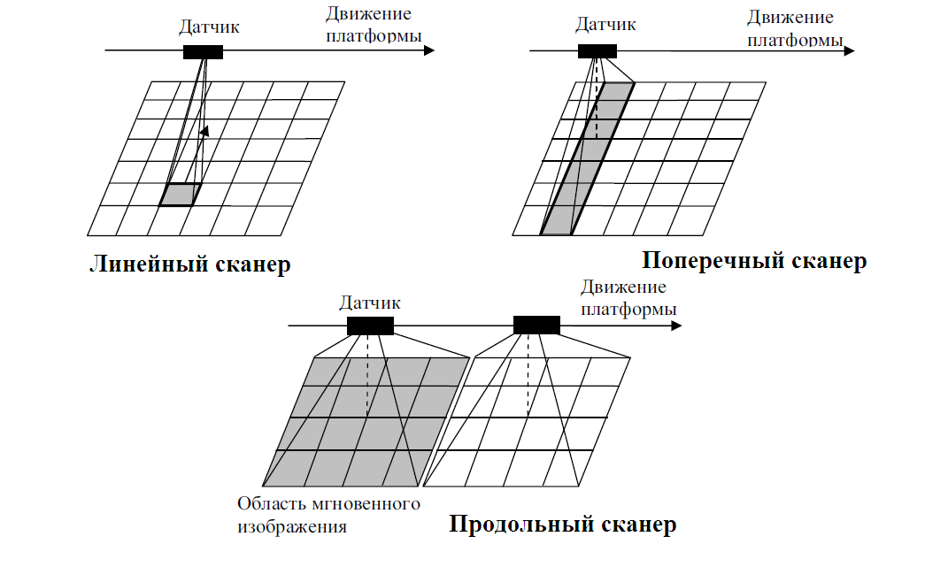
Much depends on the type of scanner, it determines the method of obtaining images. So, there are three main types of scanners:
Digital images are displayed either using an 8-bit grayscale or 24-bit scale, which is based on mixing different R, G, B shades. The original pixel range turns into a limited range by combining color values that correspond to any three channels of a multi-spectral digital image. . One pixel is displayed 256 ^ 3 RGB vectors, one vector - one color. There are other options for radiometric resolution. For example, QuickBird - 11bit / pix, Landsat-8 - 16 bit / pix.
As spectral channels are formed in optical sensors:
The beam of light received by the sensors is divided into several rays. Each beam, passing its optical path, goes through a spectral filter. Prisms and diffraction gratings can be used to separate spectral ranges.
')
The cycle of preliminary procedures for processing a snapshot includes the following:
Decryption is the process of detecting and recognizing objects and terrain phenomena in a picture. It can be either manual, that is based on visual (human) image evaluation, or machine (automatic). The last, something tells me, is of greater interest to many Habrayuzerov. Machining, in essence, comes down to different classification mechanisms. First you need to provide all the pixels (their spectral brightness) as a vector in the space of spectral features. When analyzing the quantitative relationships of the spectral brightness of different objects, the pixels are divided into classes. The classification of images is divided into classification with training and classification without training.
Classification with training assumes the presence of a reference, with the brightness of which the brightness of each pixel is compared. As a result, having several standards predetermined, we get a set of objects divided into classes. This classification only works if the objects that are shown in the image are known in advance, the classes are clearly distinguishable and their number is small.
Here are just a few of the methods that can be used in the classification with training:
Classification without training is based on the fully automatic distribution of pixels by class based on the statistics of the distribution of brightness pixel values. This type of classification is used if it is not initially known how many objects are present in the image, the number of objects is large, as a result the machine itself produces the resulting classes, and we already determine which objects to put them in line with.
All processes of preprocessing and improving the quality of images, as well as decoding, constitute a huge field for reasoning, each of them can serve as a reason for a whole article (and not just one). If anyone is interested in a specific topic, please leave your wishes in the comments for the subsequent development of the plot. Further, a post is planned on the use of various indices, such as vegetative NDVI, to improve the interpretation and identification of objects.
The article used information from the site , also from the following sources: 1 and 2 .
PS There is an opportunity to download digital data for free on the website of the US Geological Survey
For your own experiments in the processing of images there is a free demo software (albeit with some limited functions, compared to the full version, but enough for a warm-up) and one more software .
From the moment a snapshot is taken from a satellite, to being able to analyze it, it must go through a whole cycle of procedures to bring it into a form convenient for receiving and subsequent analysis of visual information.
Those who are interested in the process itself, please under the cat (traffic):
Before turning to the very essence, I would like to immediately introduce a number of
The digital image itself and the process of getting it
As everyone knows, a digital image is a matrix of pixels, the value of each of which is obtained by averaging over four components: the coordinates of space (x and y), wavelength and time.
The process of compiling the matrix itself goes this way: the solar radiation is reflected from the objects of the survey, the energy that falls on the sensor surface is fixed by it, then integrated, from which the integral pixel value is set. The integer value is obtained after converting the integral value into an electrical signal. Each pixel stores information in binary form. The more bits (memory) is allocated per pixel, the greater the number of values corresponding to one pixel, the more accurately the original discrete signal is approximated, and the more information a picture can store.
In CCD scanners, the already mentioned detectors scan the Earth and divide a continuous stream of data into pixels.
Much depends on the type of scanner, it determines the method of obtaining images. So, there are three main types of scanners:
- A linear scanner (for example, AVHRR) is the simplest, it is equipped with only one detector element.
- Transverse CCD scanner (GOES, MODIS, TM) - uses for scanning a line of detectors located along the shooting route. Parallel scanning of the Earth is carried out with each cycle of movement of the mirror.
- Longitudinal scanners (IKONOS, QuickBird, SPOT) have thousands of detectors in a CCD array, therefore, parallel scanning is carried out simply by moving the platform in orbit.
Digital images are displayed either using an 8-bit grayscale or 24-bit scale, which is based on mixing different R, G, B shades. The original pixel range turns into a limited range by combining color values that correspond to any three channels of a multi-spectral digital image. . One pixel is displayed 256 ^ 3 RGB vectors, one vector - one color. There are other options for radiometric resolution. For example, QuickBird - 11bit / pix, Landsat-8 - 16 bit / pix.
As spectral channels are formed in optical sensors:
The beam of light received by the sensors is divided into several rays. Each beam, passing its optical path, goes through a spectral filter. Prisms and diffraction gratings can be used to separate spectral ranges.
')
Preliminary procedures for image processing
The cycle of preliminary procedures for processing a snapshot includes the following:
- Radiometric correction - eliminates the variation of pixel brightness values, which occurs as a result of improper operation of detectors, the effect of relief and atmosphere.
- Atmospheric correction is a correction for the influence of the atmosphere, which determines the location of the shooting ranges at the expense of transparency windows.
- Geometric correction includes correction of such image distortions as banding, line dropping, and geocoding — linking the image so that each point of the image is given the coordinate of the corresponding point on the ground. Mathematically, geolocation is usually performed using power polynomials. The accuracy of the binding increases in the presence of reference points, then the snapshot seems to be “planted” over them. After geocoding, the brightness characteristics of an already transformed image are determined by various methods: the nearest neighbor, bilinear interpolation, bicubic convolution.
- Orthotransformation - when it eliminates image errors due to differences in the heights of the terrain, as a result, many central design flaws are eliminated in the resulting image.
The following is a process for improving image quality, including:
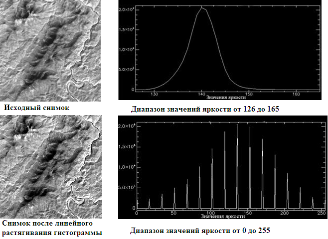
- Spectral transformations that are based on the work with the spectral chart - a graph showing the relationship between the number of pixels of the image and the values of the spectral brightness. With spectral transformations, such a parameter as contrast is changed. To enhance it, there are a number of methods, for example:
- linear stretching of the histogram, which consists in the fact that all values of brightness are assigned new values in order to cover the entire possible range from 0 to 255:
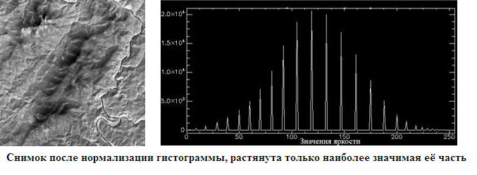
- Histogram normalization - only the most intensive (most informative) section of the diagram is stretched over the entire range of brightness values:
- Linearization of the histogram - each pixel is assigned a new brightness value, and in such a way that each brightness level has approximately the same number of pixels:
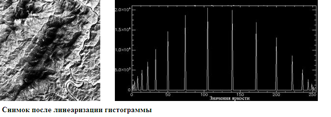
- linear stretching of the histogram, which consists in the fact that all values of brightness are assigned new values in order to cover the entire possible range from 0 to 255:
- Filtering - enhances the reproduction of objects, eliminates noise, emphasizes structural lines, smooths the image and does much more - depending on the task. The whole filtering process is based on the notion of a sliding window - a square matrix of weights (usually it is a 3 * 3 or 5 * 5 matrix). Each pixel brightness value is recalculated as follows: if a pixel is located in the center of a window moving from pixel to image pixel, then it is assigned a new value calculated from the functional dependencies of the surrounding pixels. So the window "slips" through all the pixels of the image, changing their value. Depending on the selected weights, the properties of the resulting image change. Habrayuser UnickSoft described in more detail the filtering in his post .
- Fourier transform improves image quality by decomposing it into multiple spatial-frequency components. The distribution of brightness characteristics in space is represented as a linear combination of periodic functions sin and cos with given characteristics in the frequency domain. For example, to remove noise, it is enough to reveal the frequency of their appearance.
The final stage of working with images - decoding
Decryption is the process of detecting and recognizing objects and terrain phenomena in a picture. It can be either manual, that is based on visual (human) image evaluation, or machine (automatic). The last, something tells me, is of greater interest to many Habrayuzerov. Machining, in essence, comes down to different classification mechanisms. First you need to provide all the pixels (their spectral brightness) as a vector in the space of spectral features. When analyzing the quantitative relationships of the spectral brightness of different objects, the pixels are divided into classes. The classification of images is divided into classification with training and classification without training.
Classification with training
Classification with training assumes the presence of a reference, with the brightness of which the brightness of each pixel is compared. As a result, having several standards predetermined, we get a set of objects divided into classes. This classification only works if the objects that are shown in the image are known in advance, the classes are clearly distinguishable and their number is small.
Here are just a few of the methods that can be used in the classification with training:
- Minimum distance method - pixel brightness values are considered as vectors in the space of spectral features. Between these values and the values of the vectors of the reference areas, the spectral distance is calculated as the root of the sum of the squares of the difference between the vectors of the pixel and the standard (in other words, the Euclidean distance between them). All pixels are divided into classes, depending on whether the distance between them and the standard exceeds the specified or not. So, if the distance is less, then the class is defined, the pixel can be attributed to the standard:

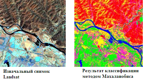
- The Mahalanobis distance method is very similar to the first method, only the classification measures not the Euclidean distance between the vectors, but the Mahalanobis distance, which takes into account the dispersion of the brightness values of the standard. In this way, if the Euclidean distance to two standards from a given pixel is equal, then the class that has a greater variance of the reference sample will win:
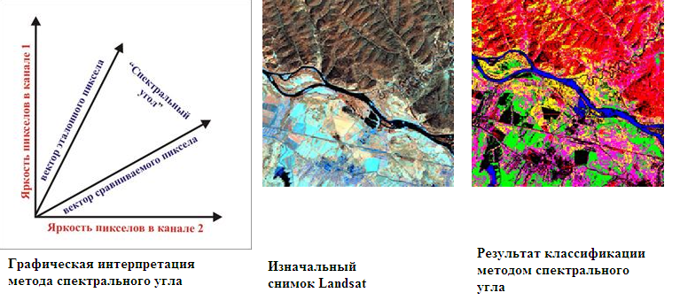
- The method of spectral angle - initially sets the maximum value of the spectral angle (the angle between the reference vector and the vector of a given pixel). The spectral angle is located, and, as with the Euclidean distance, if the angle is less than the specified one, then the pixel falls into the standard class, with which the comparison is made:
Classification without training
Classification without training is based on the fully automatic distribution of pixels by class based on the statistics of the distribution of brightness pixel values. This type of classification is used if it is not initially known how many objects are present in the image, the number of objects is large, as a result the machine itself produces the resulting classes, and we already determine which objects to put them in line with.
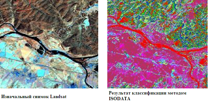
- The ISODATA (Iterative Self-Organizing Data Analysis Technique Algorithm) method is based on cluster analysis using the method of successive approximations. After considering the brightness of the pixels as vectors in the space of spectral features, the closest ones are defined in one class. For each spectral zone, statistical parameters of the brightness distribution are calculated. All pixels are divided into some n number of equal ranges, within each of which there is an average value. For each pixel of the range, the spectral distance to the average value is calculated. All pixels, the distance between which the smallest are defined in one cluster. This is the first iteration. In the second iteration and subsequent ones, the calculation of the already actual average values for each cluster takes place. Each new iteration clarifies the boundaries of future classes:
- The K-means method is similar to the previous method, with the only exception that the initial average values are set (this is possible only if the objects in the image are well readable).
All processes of preprocessing and improving the quality of images, as well as decoding, constitute a huge field for reasoning, each of them can serve as a reason for a whole article (and not just one). If anyone is interested in a specific topic, please leave your wishes in the comments for the subsequent development of the plot. Further, a post is planned on the use of various indices, such as vegetative NDVI, to improve the interpretation and identification of objects.
The article used information from the site , also from the following sources: 1 and 2 .
PS There is an opportunity to download digital data for free on the website of the US Geological Survey
For your own experiments in the processing of images there is a free demo software (albeit with some limited functions, compared to the full version, but enough for a warm-up) and one more software .
Source: https://habr.com/ru/post/210810/
All Articles