The task of changing the voice. Part 2. The physical / acoustic approach to the presentation of the speech signal
With this post we continue the cycle of articles devoted to the task of analyzing and changing a person’s voice. We briefly recall the content of the previous article :
- it was briefly told about the sound composition of speech
- such important processes as phonation and articulation were described
- a non-strict classification of the sounds of human speech was given and the characteristic features of the classes of sounds were described
- briefly identified the problems encountered in the processing of speech signals
We also outlined a bit the tasks that our division in i-Free company actually performs. The previous article was completed, the “loud” promise to describe the speech signal presentation models and to show how these models could be used to change the voice of the announcer.
')
Here we will immediately make a small reservation. The term "speech signal" can be perceived differently and often the meaning depends on the context. In the context of our work, we are interested only in the sound-acoustic properties of a speech signal, its semantic and emotional load will not be considered in this and the nearest articles.
With a creative approach to the task of changing the voice, most of the well-known models of speech signal representation are very powerful tools that allow you to do very, very much. Somehow it is not advisable to classify such undertakings, and it will take a lot of time to demonstrate “everything in a row”. In this and the next article we will confine ourselves to a brief description of the most frequently used models and somehow try to explain their physical / practical meaning. Examples of the application of these models will be shown later - in the next articles we will describe the simplest implementation of such effects as changes in gender and age of the announcer.
WARNING!

This article aims to describe a little bit the physics of sound formation in the vocal tract using a simplified model. As a result, the article contains a number of formulas and, possibly, not quite obvious transitions. The original sources are indicated in the text and, if desired, you can get acquainted with this material in more detail yourself. The models described in this article are rarely used for practical tasks of processing recorded speech, rather for research. A reader interested only in applied speech signal presentation models will be able to learn more about himself in our next article.
In order to change the properties of any signal it is not always required its exact description. Operations such as amplification, filtering, resampling (changing the sampling rate), compression , clipping can be done with only a rough knowledge of the signal being processed. With regard to the task of sound processing, such operations can be attributed to the most basic. Their use, with the exception of "extreme" cases, as a rule, does not greatly affect the perception of the processed sound. It is very difficult to get really interesting effects with their help, and beyond recognition to spoil the signal with immense use is easier than ever.
It is possible to apply some more tricky transformations, for example modulation and delay (with direct and feedback). Such well-known effects as flanger, tremolo / vibrato, chorus, phaser, wah-wah, com-filter and many others are built on these transformations and can be quite applied not only to musical instruments, but also to the voice. More details about these effects and their implementation can be found in the literature indicated at the end of the sub-clause. As mentioned in the first article, these effects give the voice a very unusual sound, but the result will not be perceived by ear as natural.
When it is required to change the voice so that the result remains at the same time “human”, the “thoughtless” conversion of the input signal will not work. A more successful approach to such a task is the analysis of the signal, the change of its parameters and the subsequent reconstruction of the new signal, the “rough” scheme for implementing the approach is shown below:
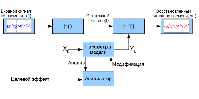
The Ƒ () symbol denotes a transformation that maps the input signal (or part of it) to a set of parameters Xk that describe certain properties of the signal. The Ƒ ^ -1 () denotes the inverse transformation from the parametric representation to the time domain, the actual "resynthesis" *. Some models describe only the most important signal properties from the point of view of this model, and so-called res. signal error - e (t). Its meaning is the difference between the input signal and the signal resynthesized using the applied model, provided that the parametric representation of the signal was not modified (e (t) = y (t) - x (t) | X_k = Y_k) **, examples will be given further. Having a parametric representation of a signal, it is possible to make a more versatile analysis and modify certain parameters, depending on the desired effect.
When analyzing a speech signal, it is always necessary to remember its property to vary greatly even at very short time intervals. Models that use time integration in their calculations, thus, can adequately describe the speech signal only at short time intervals. This directly implies the need for signal processing using similar models in small portions. Therefore, in the process of resynthesis, it is necessary to pay special attention to “sticking seams” so that the short synthesized signal fragments smoothly (without “clicks”) flow into one another.
* - the operator ^ will be denoted further by the raising to a power, ie, k ^ n - the raising of the number k to the power n.
** - the underscore will be symbolized below as subscript indexing
_______________________
Promised literature describing the "internal" device of many audio-sound effects:
The Theory and Technique of Electronic Music (Miller Puckette)
DAFX - Digital Audio Effects (edited by Udo Zolzer)
Introduction To Digital Signal Processing - Computer Musically Speaking (Tae Hong Park)
It is worth starting a conversation about speech signal models from the model of the “lowest” level, the acoustic model of the speech signal, if I may say so. Looking ahead, we will immediately say that research at this level is close to basic science and requires a very serious theoretical base and technical equipment. In our department, such work is not carried out and here this model is mentioned only for scientific and educational purposes. (Please do not react sharply to the “boring appearance” of references to the literature, their decoding will be given at the end of the article and interested readers will be able to independently investigate the issue)
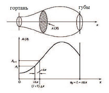
The purpose of the acoustic model is to describe the physiological device of the vocal tract of a particular person, parameterize the process of articulation in time and reflect the influence of these parameters on the air flow passing through the vocal tract. As a basic work, many authors refer to [1], where M. Portnoff studied the question of approximating a human speech tract using a pipe with an uneven time-varying cross-sectional area (illustration below).
The basic differential equations describing the relationship of pressure and air velocity in this pipe [2], [3] are presented below. In appearance, they do not seem so “scary” (if you do not disclose in detail each member of the equation):

where p = p (x, t) is the pressure change depending on time t and coordinates of point x in the pipe, u = u (x, t) is the volume velocity of the air flow in the pipe, ρ is the density of air in the pipe, c is the speed sound, A = A (x, t) - the cross-sectional area of the pipe at the point x at the moment of time t. Total pipe length - l.
These equations have no algebraic solution except for the simplest cases with strict restrictions on the initial / final conditions [3]. To find numerical solutions, it is necessary to obtain the values of pressure and air velocity at the starting and ending points of the vocal tract - the larynx and lips, respectively. Nevertheless, the uncertainty of the values of the function A (x, t) remains a big problem. As stated in [4], advances in the field of three-dimensional tomography make it possible to make significant refinements to the relationship of the area of the vocal tract and its acoustic characteristics. However, even knowing fully the behavior of A (x, t), or in the case of its stationarity in time (which is valid when analyzing short vocalized segments), it is still necessary to make a large number of assumptions in order to obtain some practically useful model. Factors that need to be considered when modeling the process of articulation using this acoustic model [3]:
1) Knowledge of the behavior of A (x, t) in time (unique for each speaker)
2) Sound energy losses due to heat transfer and viscous friction in the vocal tract
3) Losses associated with the elasticity of the walls of the vocal tract (their compliance with incoming air pulses)
4) Radiation of sound in the lips area
5) The influence of the nasopharynx, as an additional resonator / sound emitter
6) The process of excitation of the initial sound waves (phonation), which is also unique for each individual person
Each of these factors is a separate topic for serious research. If you go back to the task of changing the voice using an approach with analysis and resynthesis, then to apply this model, you need to restore a large number of physiological parameters of the speaker’s speech path from the incoming signal. Experts call finding the vocal tract parameters and / or articulation parameters using the existing audio signal a reverse speech problem ([5]). These tasks are ill-conditioned and for their exact solution they require large restrictions on the values of the desired parameters, or their plausible initial approximations, which can be obtained using specialized measurements.
From the point of view of sound processing, obtaining a physically-accurate model of a person’s vocal tract and its articulation parameters is of greatest importance for:
- forensic examination
- medical diagnostics
- speech synthesis systems (text-to-speech systems)
In real-time sound processing, accurate physical / acoustic modeling of sound production is hardly possible without any prior knowledge of the speaker's speech path. For this reason, it is hard to imagine the application of this approach to work with unknown voices. Although theoretically it is the physico-acoustic approach that should, with a competent implementation, give the most plausible sound, since it is a direct simulation of the processes occurring during sound production.
Having made some assumptions, it is possible to obtain a simplified approximation of the vocal tract from the model described above, and the frequency response of this approximation is quite close to real measurements. A good description of this simplified model is given in [3]. The following is the main point, with an emphasis on the implied, but not explicitly explained in [3] details. The above assumptions are as follows:
a) For “long” sound waves (whose frequency is less than 4000 Hz, respectively, a length of ~ 9 cm or more), it is possible to neglect the turns in the vocal tract and present it as an elongated tube (as in the previous figure). Such an approach is close to analyzing the acoustics of many wind instruments, where only propagation of longitudinal sound waves is considered.
b) It is possible to neglect the losses due to viscous friction and heat conduction. These losses are significantly manifested only in the region of high frequencies, and their influence in comparison with the losses in the emission of sound is small.
c) The losses associated with the elasticity of the walls of the vocal tract are neglected.
d) The radiating surface (mouth and / or nose) is approximated by a hole on the plane, not on the sphere.
e) To solve differential equations describing the relationship between air volume velocity and pressure, restrictions are imposed on the boundary conditions:
- the sound source in the area of the larynx (Glottis) u_G (0, t) is not subject to pressure fluctuations in the vocal tract,
- pressure at the exit of the vocal tract in the region of the lips (Lips) p_L (l, t) is constant.
f) The cross-sectional area A (x, t) is approximated by a discrete function, see figure below. The speech path, therefore, is the concatenation of pipes of different diameters. At the time of the analysis, it is assumed that A (x, t) is stationary in time, which is valid for short time intervals.

To find the frequency response of this system, we need to find the ratio of the frequency response of the signal at the system output U_n (w) to the frequency response of the signal at the input of the system U_1 (w). To do this, the input signal should be presented as a complex exponential with an arbitrary frequency and some amplitude characteristic (U_G (w) * exp (jwt)). After that, it is necessary to apply equations (1) sequentially for each pipe in the system. At the pipe joints, it is possible to apply the principle of continuity of functions u (x, t) and p (x, t) in space. More simple words:
1) Suppose that analyzed the 1st and 2nd segments
2) the pressure and air velocity at the very end of the 1st segment should be equal to the pressure and air velocity at the very beginning of the 2nd segment
3) we obtain the relations:
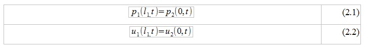
Relations (2) will be valid both for the functions p (x, t) and u (x, t), and for their frequency characteristics P (x, w) and U (x, w).
The analysis can be carried out from beginning to end (from the larynx to the lips), and vice versa. The second option is even simpler. For complete happiness, it is only necessary to apply the “most extreme” conditions:

The value Z_L (w) is called the radiation impedance and in the case of the analysis of human speech, when the radiating surface is approximated by a small hole on a large plane (condition (d)) it can be expressed as a function of frequency and some predetermined constants L_L and R_L. The value of Z_G (w) is the acoustic impedance in the larynx and can also be calculated using some predefined constants L_G and R_G. U_0 (w) is the frequency response of the signal at the output of the larynx, which we conditionally assumed for the frequency analysis of our model by some complex exponential.
Using solutions for differential equations (1) and applying the condition of continuity of pressure and volume velocity of air in space, it becomes possible to pass through the entire "chain" of pipes and express the initial velocity of the air flow U_G (w) as a function of the final velocity U_L (w) or vice versa:

where f_k is a certain function that depends both on the solutions of equations (1) for the k-th pipe, and on the length / area of the k-th pipe. After this, it is comparatively easy to find the relation of “entrance” to “exit”.
All described steps are valid only under assumptions a) -e). The resulting frequency response, with an adequate discrete approximation of the vocal tract (A_k and l_k, k = 1: n), adequately describes the formant characteristics of various vowels and non-nasal consonant sounds. To describe the nasal sounds, the system must become more complex, since it is necessary to take into account the additional radiating surface and the branching of the vocal tract that occurs when the soft palate is sinking.
Losses associated with heat transfer, viscous friction and elasticity of the vocal tract can be adequately taken into account in this model, but then the basic differential equations (the form of the function A (x, t) becomes more complicated) and the boundary conditions become somewhat more complicated.
To implement sound effects, the use of this model implies an assessment of the A_k and l_k values from the signal being processed, their modification and the subsequent synthesis of a new sound. To solve the inverse problem of estimating A_k and l_k by the input signal, it is necessary to know the excitation signal that passed through the speech path at the time of analysis, or at least to have its plausible approximation. To approximate the excitation signal of a voiced speech fragment, there are a considerable number of models, but for their use it is necessary, in turn, to determine the appropriate choice of the model and the selection of its parameters for the signal being processed, which is also not always a trivial task. Again, there are methods that allow recovering the voice path excitation signal from the sound being processed with various kinds of errors.
Even if there is a good approximation of the excitation signal, finding the values of A_k and l_k requires solving a system of nonlinear equations, which in turn draws numerical methods and the search for optimal values with all the consequences. What has been said conceptually (NOT MATHEMATICALLY STRICTLY!) Is depicted in the figure below:
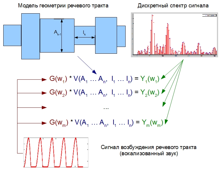
In this figure, Y (w_k) and G (w_k) is the discrete spectrum of the signal being processed and its excitation signal, respectively. V (A, I) is a model of the frequency characteristics of the vocal tract, depending on the desired A_k and l_k.
The implementation of a system capable of doing all of the above in the absence of any prior knowledge of the signal seems to be quite a challenge. Additional difficulties arise when trying to make such a system work with noisy signals in real time.
In general, we can conclude that such a model has more value for text-to-speech synthesis problems. The analysis of the unknown input signal with the help of such a model is a rather dubious pleasure. There is an alternative look at this model, making it more suitable for "our" purposes.
To begin with, we will immediately introduce one more additional constraint on the model considered in the previous paragraph:
All lengths of the tubes that make up the vocal tract are taken equal to each other:
l_1 = l_2 = ... = l_n = LEN
Next, you should turn to the acoustics of pipes and remember that longitudinal sound waves tend to be reflected from the open end of the pipe. In other words, the function of the volume velocity of the air flow is a function of two air waves propagating in different directions: u (t, x) = f (u + (t, x), u- (t, x)). Indices + and - we will denote sound waves going in the forward (from the larynx to the lips) and opposite directions, respectively. The above is schematically illustrated below:
It is important to remember that only the diagram is shown. In fact, the sound does not move forward along the top and back along the bottom of the pipe. In order to somehow imagine how this is actually happening, you can turn to a wonderful illustration from cnx.org, which shows a standing acoustic wave in an ideal tube.
This is also confirmed by the fact that equations (1) have general solutions of the form:

Recall that ρ is the density of air in the pipe, c is the speed of sound, A = A (x, t) is the cross-sectional area of the pipe at point x at time t. u + (x, t) is the space velocity of air going in the forward direction, u- (x, t) is in the opposite direction.
As stated in [3], these solutions can be derived by applying the theory of analysis of electrical circuits, assuming an analogy: pressure p is voltage in circuit U; air flow rate u current in circuit I; acoustic inductance ρ / A inductance L; acoustic capacitance A / (ρc ^ 2) capacitance C.
Equations (5) are valid for each pipe that makes up our approximation of the vocal tract. Now, knowing the general form of solutions of equations (1), we apply the condition of continuity of pressure and air velocity in space and, denoting by k the index of the analyzed pipe, we can say that
Having made a number of algebraic transformations (for details, refer to [3]), it is possible to show that:
The coefficient r_k in this system is called the reflection coefficient, its numerical value can be expressed as:

l_k/c, (6), (7) , k- . . . LEN, τ , , LEN.
(7), / . :
— / ( r_k).
t T_s. , τ . . 350 / 0.175 (17.5 ), , 0.0005 . , 10 . τ 0.00005 . , , Ts, : F_s = 1/T_s = 20 . — «» ( ). , . [3], , , 2τ, . . , 2τ. «» - , ( ) . , [3]. , :
— Z-
— z^(-1)
, 3- :
(3). (3) (1+r_G)/2 (1+r_L) . z^(3/2) «» — 3 z^(-1/2) «» z^(3/2).
«» , (1) (7), t . , , — A_k. , A_k, , , ( ).
, , Z- , ([2], [3]):

G(z) — , V(z) — ( A(x,t)), R(z) – .
, G(z) R(z) ( R(z), ). V(z) . G(z), .. . G(z) .
, — . , , , .
text-to-speech. , «» .
, :
— LPC ( «» )
— ( )
— HPN-
________________________
:
[1] MR Portnoff, A Quasi-One-Dimensional Digital Simulation for Time-Varying Vocal Tract
[2] NR Raajan, TR Sivaramakrishnan and Y. Venkatramani, Mathematical Modeling of Speech Production and Its Application to Noise Cancellation (Chapter 3 from Speech Enhancement, Modeling and Recognition – Algorithms and Applications)
[3] LR Rabiner, RW Schafer, Digital Processing of Speech Signals
[4] . . ,
[5] .., .., .
- it was briefly told about the sound composition of speech
- such important processes as phonation and articulation were described
- a non-strict classification of the sounds of human speech was given and the characteristic features of the classes of sounds were described
- briefly identified the problems encountered in the processing of speech signals
We also outlined a bit the tasks that our division in i-Free company actually performs. The previous article was completed, the “loud” promise to describe the speech signal presentation models and to show how these models could be used to change the voice of the announcer.
')
Here we will immediately make a small reservation. The term "speech signal" can be perceived differently and often the meaning depends on the context. In the context of our work, we are interested only in the sound-acoustic properties of a speech signal, its semantic and emotional load will not be considered in this and the nearest articles.
With a creative approach to the task of changing the voice, most of the well-known models of speech signal representation are very powerful tools that allow you to do very, very much. Somehow it is not advisable to classify such undertakings, and it will take a lot of time to demonstrate “everything in a row”. In this and the next article we will confine ourselves to a brief description of the most frequently used models and somehow try to explain their physical / practical meaning. Examples of the application of these models will be shown later - in the next articles we will describe the simplest implementation of such effects as changes in gender and age of the announcer.
WARNING!
This article aims to describe a little bit the physics of sound formation in the vocal tract using a simplified model. As a result, the article contains a number of formulas and, possibly, not quite obvious transitions. The original sources are indicated in the text and, if desired, you can get acquainted with this material in more detail yourself. The models described in this article are rarely used for practical tasks of processing recorded speech, rather for research. A reader interested only in applied speech signal presentation models will be able to learn more about himself in our next article.
Sound effects and why do we need speech representation models?
In order to change the properties of any signal it is not always required its exact description. Operations such as amplification, filtering, resampling (changing the sampling rate), compression , clipping can be done with only a rough knowledge of the signal being processed. With regard to the task of sound processing, such operations can be attributed to the most basic. Their use, with the exception of "extreme" cases, as a rule, does not greatly affect the perception of the processed sound. It is very difficult to get really interesting effects with their help, and beyond recognition to spoil the signal with immense use is easier than ever.
It is possible to apply some more tricky transformations, for example modulation and delay (with direct and feedback). Such well-known effects as flanger, tremolo / vibrato, chorus, phaser, wah-wah, com-filter and many others are built on these transformations and can be quite applied not only to musical instruments, but also to the voice. More details about these effects and their implementation can be found in the literature indicated at the end of the sub-clause. As mentioned in the first article, these effects give the voice a very unusual sound, but the result will not be perceived by ear as natural.
When it is required to change the voice so that the result remains at the same time “human”, the “thoughtless” conversion of the input signal will not work. A more successful approach to such a task is the analysis of the signal, the change of its parameters and the subsequent reconstruction of the new signal, the “rough” scheme for implementing the approach is shown below:
The Ƒ () symbol denotes a transformation that maps the input signal (or part of it) to a set of parameters Xk that describe certain properties of the signal. The Ƒ ^ -1 () denotes the inverse transformation from the parametric representation to the time domain, the actual "resynthesis" *. Some models describe only the most important signal properties from the point of view of this model, and so-called res. signal error - e (t). Its meaning is the difference between the input signal and the signal resynthesized using the applied model, provided that the parametric representation of the signal was not modified (e (t) = y (t) - x (t) | X_k = Y_k) **, examples will be given further. Having a parametric representation of a signal, it is possible to make a more versatile analysis and modify certain parameters, depending on the desired effect.
When analyzing a speech signal, it is always necessary to remember its property to vary greatly even at very short time intervals. Models that use time integration in their calculations, thus, can adequately describe the speech signal only at short time intervals. This directly implies the need for signal processing using similar models in small portions. Therefore, in the process of resynthesis, it is necessary to pay special attention to “sticking seams” so that the short synthesized signal fragments smoothly (without “clicks”) flow into one another.
* - the operator ^ will be denoted further by the raising to a power, ie, k ^ n - the raising of the number k to the power n.
** - the underscore will be symbolized below as subscript indexing
_______________________
Promised literature describing the "internal" device of many audio-sound effects:
The Theory and Technique of Electronic Music (Miller Puckette)
DAFX - Digital Audio Effects (edited by Udo Zolzer)
Introduction To Digital Signal Processing - Computer Musically Speaking (Tae Hong Park)
Physical modeling of sound in speech. Acoustic model of the vocal tract.
It is worth starting a conversation about speech signal models from the model of the “lowest” level, the acoustic model of the speech signal, if I may say so. Looking ahead, we will immediately say that research at this level is close to basic science and requires a very serious theoretical base and technical equipment. In our department, such work is not carried out and here this model is mentioned only for scientific and educational purposes. (Please do not react sharply to the “boring appearance” of references to the literature, their decoding will be given at the end of the article and interested readers will be able to independently investigate the issue)
The purpose of the acoustic model is to describe the physiological device of the vocal tract of a particular person, parameterize the process of articulation in time and reflect the influence of these parameters on the air flow passing through the vocal tract. As a basic work, many authors refer to [1], where M. Portnoff studied the question of approximating a human speech tract using a pipe with an uneven time-varying cross-sectional area (illustration below).
The basic differential equations describing the relationship of pressure and air velocity in this pipe [2], [3] are presented below. In appearance, they do not seem so “scary” (if you do not disclose in detail each member of the equation):
where p = p (x, t) is the pressure change depending on time t and coordinates of point x in the pipe, u = u (x, t) is the volume velocity of the air flow in the pipe, ρ is the density of air in the pipe, c is the speed sound, A = A (x, t) - the cross-sectional area of the pipe at the point x at the moment of time t. Total pipe length - l.
These equations have no algebraic solution except for the simplest cases with strict restrictions on the initial / final conditions [3]. To find numerical solutions, it is necessary to obtain the values of pressure and air velocity at the starting and ending points of the vocal tract - the larynx and lips, respectively. Nevertheless, the uncertainty of the values of the function A (x, t) remains a big problem. As stated in [4], advances in the field of three-dimensional tomography make it possible to make significant refinements to the relationship of the area of the vocal tract and its acoustic characteristics. However, even knowing fully the behavior of A (x, t), or in the case of its stationarity in time (which is valid when analyzing short vocalized segments), it is still necessary to make a large number of assumptions in order to obtain some practically useful model. Factors that need to be considered when modeling the process of articulation using this acoustic model [3]:
1) Knowledge of the behavior of A (x, t) in time (unique for each speaker)
2) Sound energy losses due to heat transfer and viscous friction in the vocal tract
3) Losses associated with the elasticity of the walls of the vocal tract (their compliance with incoming air pulses)
4) Radiation of sound in the lips area
5) The influence of the nasopharynx, as an additional resonator / sound emitter
6) The process of excitation of the initial sound waves (phonation), which is also unique for each individual person
Each of these factors is a separate topic for serious research. If you go back to the task of changing the voice using an approach with analysis and resynthesis, then to apply this model, you need to restore a large number of physiological parameters of the speaker’s speech path from the incoming signal. Experts call finding the vocal tract parameters and / or articulation parameters using the existing audio signal a reverse speech problem ([5]). These tasks are ill-conditioned and for their exact solution they require large restrictions on the values of the desired parameters, or their plausible initial approximations, which can be obtained using specialized measurements.
From the point of view of sound processing, obtaining a physically-accurate model of a person’s vocal tract and its articulation parameters is of greatest importance for:
- forensic examination
- medical diagnostics
- speech synthesis systems (text-to-speech systems)
In real-time sound processing, accurate physical / acoustic modeling of sound production is hardly possible without any prior knowledge of the speaker's speech path. For this reason, it is hard to imagine the application of this approach to work with unknown voices. Although theoretically it is the physico-acoustic approach that should, with a competent implementation, give the most plausible sound, since it is a direct simulation of the processes occurring during sound production.
More "down to earth" approach. Simplified acoustic model of the vocal tract.
Having made some assumptions, it is possible to obtain a simplified approximation of the vocal tract from the model described above, and the frequency response of this approximation is quite close to real measurements. A good description of this simplified model is given in [3]. The following is the main point, with an emphasis on the implied, but not explicitly explained in [3] details. The above assumptions are as follows:
a) For “long” sound waves (whose frequency is less than 4000 Hz, respectively, a length of ~ 9 cm or more), it is possible to neglect the turns in the vocal tract and present it as an elongated tube (as in the previous figure). Such an approach is close to analyzing the acoustics of many wind instruments, where only propagation of longitudinal sound waves is considered.
b) It is possible to neglect the losses due to viscous friction and heat conduction. These losses are significantly manifested only in the region of high frequencies, and their influence in comparison with the losses in the emission of sound is small.
c) The losses associated with the elasticity of the walls of the vocal tract are neglected.
d) The radiating surface (mouth and / or nose) is approximated by a hole on the plane, not on the sphere.
e) To solve differential equations describing the relationship between air volume velocity and pressure, restrictions are imposed on the boundary conditions:
- the sound source in the area of the larynx (Glottis) u_G (0, t) is not subject to pressure fluctuations in the vocal tract,
- pressure at the exit of the vocal tract in the region of the lips (Lips) p_L (l, t) is constant.
f) The cross-sectional area A (x, t) is approximated by a discrete function, see figure below. The speech path, therefore, is the concatenation of pipes of different diameters. At the time of the analysis, it is assumed that A (x, t) is stationary in time, which is valid for short time intervals.
To find the frequency response of this system, we need to find the ratio of the frequency response of the signal at the system output U_n (w) to the frequency response of the signal at the input of the system U_1 (w). To do this, the input signal should be presented as a complex exponential with an arbitrary frequency and some amplitude characteristic (U_G (w) * exp (jwt)). After that, it is necessary to apply equations (1) sequentially for each pipe in the system. At the pipe joints, it is possible to apply the principle of continuity of functions u (x, t) and p (x, t) in space. More simple words:
1) Suppose that analyzed the 1st and 2nd segments
2) the pressure and air velocity at the very end of the 1st segment should be equal to the pressure and air velocity at the very beginning of the 2nd segment
3) we obtain the relations:
Relations (2) will be valid both for the functions p (x, t) and u (x, t), and for their frequency characteristics P (x, w) and U (x, w).
The analysis can be carried out from beginning to end (from the larynx to the lips), and vice versa. The second option is even simpler. For complete happiness, it is only necessary to apply the “most extreme” conditions:
The value Z_L (w) is called the radiation impedance and in the case of the analysis of human speech, when the radiating surface is approximated by a small hole on a large plane (condition (d)) it can be expressed as a function of frequency and some predetermined constants L_L and R_L. The value of Z_G (w) is the acoustic impedance in the larynx and can also be calculated using some predefined constants L_G and R_G. U_0 (w) is the frequency response of the signal at the output of the larynx, which we conditionally assumed for the frequency analysis of our model by some complex exponential.
Using solutions for differential equations (1) and applying the condition of continuity of pressure and volume velocity of air in space, it becomes possible to pass through the entire "chain" of pipes and express the initial velocity of the air flow U_G (w) as a function of the final velocity U_L (w) or vice versa:
where f_k is a certain function that depends both on the solutions of equations (1) for the k-th pipe, and on the length / area of the k-th pipe. After this, it is comparatively easy to find the relation of “entrance” to “exit”.
All described steps are valid only under assumptions a) -e). The resulting frequency response, with an adequate discrete approximation of the vocal tract (A_k and l_k, k = 1: n), adequately describes the formant characteristics of various vowels and non-nasal consonant sounds. To describe the nasal sounds, the system must become more complex, since it is necessary to take into account the additional radiating surface and the branching of the vocal tract that occurs when the soft palate is sinking.
Losses associated with heat transfer, viscous friction and elasticity of the vocal tract can be adequately taken into account in this model, but then the basic differential equations (the form of the function A (x, t) becomes more complicated) and the boundary conditions become somewhat more complicated.
To implement sound effects, the use of this model implies an assessment of the A_k and l_k values from the signal being processed, their modification and the subsequent synthesis of a new sound. To solve the inverse problem of estimating A_k and l_k by the input signal, it is necessary to know the excitation signal that passed through the speech path at the time of analysis, or at least to have its plausible approximation. To approximate the excitation signal of a voiced speech fragment, there are a considerable number of models, but for their use it is necessary, in turn, to determine the appropriate choice of the model and the selection of its parameters for the signal being processed, which is also not always a trivial task. Again, there are methods that allow recovering the voice path excitation signal from the sound being processed with various kinds of errors.
Even if there is a good approximation of the excitation signal, finding the values of A_k and l_k requires solving a system of nonlinear equations, which in turn draws numerical methods and the search for optimal values with all the consequences. What has been said conceptually (NOT MATHEMATICALLY STRICTLY!) Is depicted in the figure below:
In this figure, Y (w_k) and G (w_k) is the discrete spectrum of the signal being processed and its excitation signal, respectively. V (A, I) is a model of the frequency characteristics of the vocal tract, depending on the desired A_k and l_k.
The implementation of a system capable of doing all of the above in the absence of any prior knowledge of the signal seems to be quite a challenge. Additional difficulties arise when trying to make such a system work with noisy signals in real time.
In general, we can conclude that such a model has more value for text-to-speech synthesis problems. The analysis of the unknown input signal with the help of such a model is a rather dubious pleasure. There is an alternative look at this model, making it more suitable for "our" purposes.
The speech path as a discrete filter
To begin with, we will immediately introduce one more additional constraint on the model considered in the previous paragraph:
All lengths of the tubes that make up the vocal tract are taken equal to each other:
l_1 = l_2 = ... = l_n = LEN
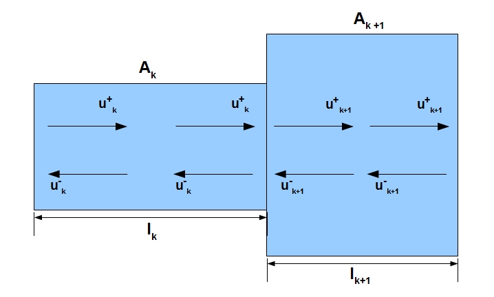
Next, you should turn to the acoustics of pipes and remember that longitudinal sound waves tend to be reflected from the open end of the pipe. In other words, the function of the volume velocity of the air flow is a function of two air waves propagating in different directions: u (t, x) = f (u + (t, x), u- (t, x)). Indices + and - we will denote sound waves going in the forward (from the larynx to the lips) and opposite directions, respectively. The above is schematically illustrated below:
It is important to remember that only the diagram is shown. In fact, the sound does not move forward along the top and back along the bottom of the pipe. In order to somehow imagine how this is actually happening, you can turn to a wonderful illustration from cnx.org, which shows a standing acoustic wave in an ideal tube.
This is also confirmed by the fact that equations (1) have general solutions of the form:
Recall that ρ is the density of air in the pipe, c is the speed of sound, A = A (x, t) is the cross-sectional area of the pipe at point x at time t. u + (x, t) is the space velocity of air going in the forward direction, u- (x, t) is in the opposite direction.
As stated in [3], these solutions can be derived by applying the theory of analysis of electrical circuits, assuming an analogy: pressure p is voltage in circuit U; air flow rate u current in circuit I; acoustic inductance ρ / A inductance L; acoustic capacitance A / (ρc ^ 2) capacitance C.
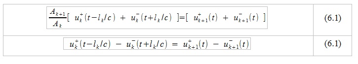
Equations (5) are valid for each pipe that makes up our approximation of the vocal tract. Now, knowing the general form of solutions of equations (1), we apply the condition of continuity of pressure and air velocity in space and, denoting by k the index of the analyzed pipe, we can say that
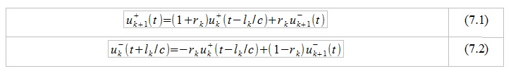
Having made a number of algebraic transformations (for details, refer to [3]), it is possible to show that:
The coefficient r_k in this system is called the reflection coefficient, its numerical value can be expressed as:
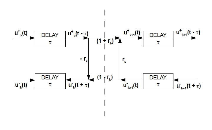
l_k/c, (6), (7) , k- . . . LEN, τ , , LEN.
(7), / . :
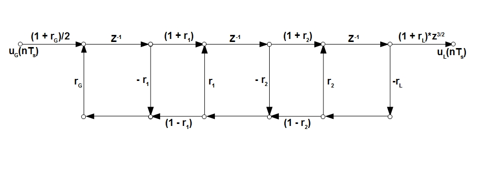
— / ( r_k).
t T_s. , τ . . 350 / 0.175 (17.5 ), , 0.0005 . , 10 . τ 0.00005 . , , Ts, : F_s = 1/T_s = 20 . — «» ( ). , . [3], , , 2τ, . . , 2τ. «» - , ( ) . , [3]. , :
— Z-
— z^(-1)
, 3- :
(3). (3) (1+r_G)/2 (1+r_L) . z^(3/2) «» — 3 z^(-1/2) «» z^(3/2).
«» , (1) (7), t . , , — A_k. , A_k, , , ( ).
findings
, , Z- , ([2], [3]):
G(z) — , V(z) — ( A(x,t)), R(z) – .
, G(z) R(z) ( R(z), ). V(z) . G(z), .. . G(z) .
, — . , , , .
text-to-speech. , «» .
, :
— LPC ( «» )
— ( )
— HPN-
________________________
:
[1] MR Portnoff, A Quasi-One-Dimensional Digital Simulation for Time-Varying Vocal Tract
[2] NR Raajan, TR Sivaramakrishnan and Y. Venkatramani, Mathematical Modeling of Speech Production and Its Application to Noise Cancellation (Chapter 3 from Speech Enhancement, Modeling and Recognition – Algorithms and Applications)
[3] LR Rabiner, RW Schafer, Digital Processing of Speech Signals
[4] . . ,
[5] .., .., .
Source: https://habr.com/ru/post/210646/
All Articles