Building a SARIMA Model with Python + R

Introduction

Good afternoon, dear readers.
After writing a previous post about analyzing time series in Python, I decided to correct the comments that were indicated in the comments, but when I corrected them, I ran into a number of problems, for example, when constructing a seasonal ARIMA model, because I did not find a similar function in the statsmodels package. In the end, I decided to use the functions from R for this, and the searches led me to the rpy2 library which allows using functions from the libraries of the mentioned language.
Many may have the question "why is this necessary?", Because it's easier to just take R and do all the work in it. I fully agree with this statement, but it seems to me that if the data requires preprocessing, then it is easier to produce it in Python , and using R capabilities, if necessary, for analysis.
In addition, it will be shown how to integrate the results of the R function in IPython Notebook.

Install and configure Rpy2

To get started, you need to install rpy2. You can do this with the command:

pip install rpy2 

It should be noted that, for the work of this library, the installed language R is necessary. You can download it from off. site .
The next thing you need to do is add the necessary system variables. For Windows, add the following variables:

• PATH - the path to R.dll and to R.exe
  
• R_HOME - the path to the folder where R is installed
  
• R_USER - username under which windows is loaded
  

It was also installed on Mac OS X, there was no need for these manipulations.

Beginning of work

So, if you are working in IPython Notebook , you need to add a statement:
')

 %load_ext rmagic 

This extension allows you to call some functions of R via rpy2 , and outputs the result directly to the IPython Notebook console, which is very convenient (it will be shown below how to do this). Read more here .
Now let's load the necessary libraries:

 from pandas import read_csv, DataFrame, Series import statsmodels.api as sm import rpy2.robjects as R from rpy2.robjects.packages import importr import pandas.rpy.common as com from pandas import date_range 

Now, as in the previous article, load the data and proceed to the weekly intervals:

 dataset = read_csv('DataSets/tovar_moving.csv',';', index_col=['date'], parse_dates=['date'], dayfirst=True) otg = dataset.qty w = otg.resample('w', how='sum') w.plot(figsize=(12,6))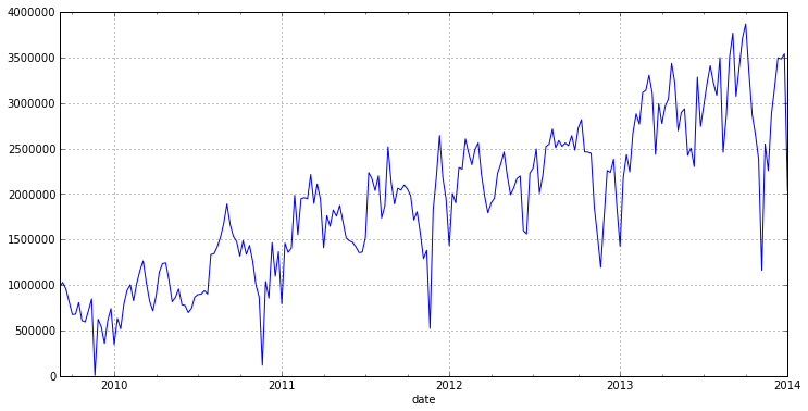 

So, from the graph you can see the annual seasonality (52 weeks) and a pronounced trend. Therefore, before building a model, we need to get rid of the trend and seasonality.

Preliminary data analysis

So for starters, let's shuffle up the original series to align the values:

 w_log = log(w) w_log.plot(figsize=(12,6))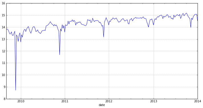 

As you can see, we have seasonality in the graph and, accordingly, the series is not stationary. Let us verify this with the help of the Dickey-Fuller test , which tests the hypothesis about the presence of unit roots and, accordingly, if they exist, the series will be non-stationary. How to conduct this test using the statsmodels library, I showed last time. Now I will demonstrate how this can be done using the adf.test () function from R.
So, this function is in the R-th library tseries . It is intended for the analysis of time series and is set additionally. You can load the required library using the importr () function.

 stats = importr('stats') tseries = importr('tseries') 

You may notice that in addition to tseries , we also loaded the stats library. We need it for type conversion.
Now it is necessary to transfer data from the Python type to the type that is understandable by R. You can do this using the function convert_to_r_dataframe (), the input of which is the DataFrame, and the output is a vector for R.

 r_df = com.convert_to_r_dataframe(DataFrame(w_log)) 

So, the vector is the next step: you need to translate it into a time series format. For this, there is a ts () function in R, its call will look like this:

 y = stats.ts(r_df) 

Preliminary data preparation is completed and we can call the function we need:

 ad = tseries.adf_test(y, alternative="stationary", k=52) 

As parameters, it is transmitted the time series and the number of lags for which the test will be calculated. In economic models, it is customary to take this value equal to the year; our data is weekly, and there are 52 weeks in a year, so the parameter has such a value.
Now the ad variable contains an R-object. Its structure is described in the form of a list, the description of which I could not find. Therefore, using visual analysis, I wrote code that displays the result of the function in a clear form:

 a = ad.names[:5] {ad.names[i]:ad[i][0] for i in xrange(len(a))} 

{'alternative': 'stationary',
'method': 'Augmented Dickey-Fuller Test',
'p.value': 0.23867869477446427,
'parameter': 52.0,
'statistic': -2.8030060277420006}

Based on the test results, the initial series is not stationary. Since the hypothesis of the presence of unit roots is accepted with a small probability, and, accordingly, the series is not stationary. We now check for stationarity a series of first differences.
First we get them using Python, and then we apply the ADF test:

 diff1lev = w.diff(periods=1).dropna() print 'p.value: %f' % sm.tsa.adfuller(diff1lev, maxlag=52)[1] 

p.value: 0.000000

 diff1lev.plot(figsize=(12,6)) 

A number of first differences, according to the test results, turned out to be stationary. A schedule helps us make sure that the trend is missing. It remains to get rid of seasonality.
For this you need to take the seasonal difference from our resulting series. Read more here . If the resulting series will be stationary, it will be necessary to knit its first difference and check it.

 diff1lev_season = diff1lev.diff(52).dropna() 

Test it for stationarity using the ADF test from R:

 r_df = com.convert_to_r_dataframe(DataFrame(diff1lev_season)) y = stats.ts(r_df) ad = tseries.adf_test(y, alternative="stationary", k=52) a = ad.names[:5] {ad.names[i]:ad[i][0] for i in xrange(len(a))} 

{'alternative': 'stationary',
'method': 'Augmented Dickey-Fuller Test',
'p.value': 0.551977997289418,
'parameter': 52.0,
'statistic': -2.0581183466564776}

So, the series is not stationary, take its first differences:

 diff1lev_season1lev = diff1lev_season.diff().dropna() print 'p.value: %f' % sm.tsa.adfuller(diff1lev_season1lev, maxlag=52)[1] 

p.value: 0.000395

The resulting series is stationary. Now you can go to build a model

Build a model.

So, the preliminary analysis is completed, and we can proceed to the construction of the seasonal ARIMA (SARIMA) model .
General view of this model
In this model, the parameters indicate the following:

• - model order
• - the order of integration of the source data
• - model order
• - the order of the seasonal component
• - the order of integration of the seasonal component
• - the order of the seasonal component
• - seasonality dimension (month, quarter, etc.)

How to determine p , d , q , I showed last time. Now I will describe to determine the order of the seasonal components of P , D , Q.
Let's start with the definition of the parameter D. It determines the order of integration of the seasonal difference, i.e. in our case it is equal to 1 . To determine P and Q, we still need to construct the ACF and PACF correlograms .

 fig = plt.figure(figsize=(12,8)) ax1 = fig.add_subplot(211) fig = sm.graphics.tsa.plot_acf(diff1lev_season1lev.values.squeeze(), lags=150, ax=ax1) ax2 = fig.add_subplot(212) fig = sm.graphics.tsa.plot_pacf(diff1lev_season1lev, lags=150, ax=ax2)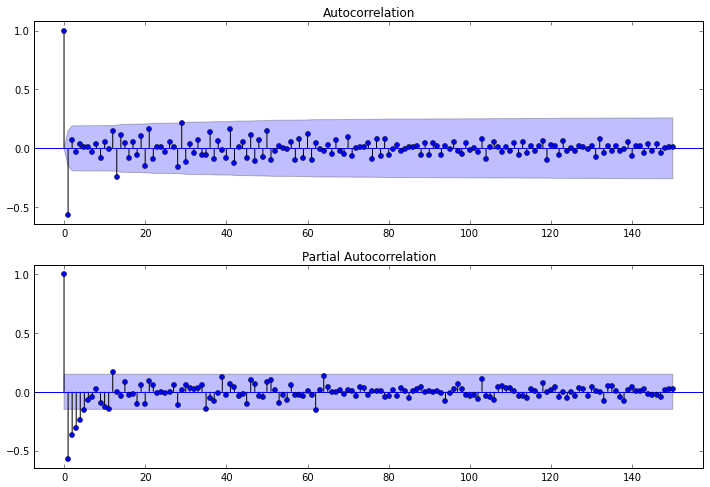 

From the PACF, you can see that the order of AR is p = 4 , and by ACF it is clear that the order of MA q = 13 , since 13 lag is the last lag different from 0.
We now turn to the seasonal components. To evaluate them, one should look at the lags multiple to the size of the seasonality, i.e. if, for our example, seasonality is 52, then lags 52, 104, 156, ... should be considered.
In our case, the parameters P and Q will be equal to 0 (this can be seen if you look at the ACF and PACF on the above lags).
As a result of our research, we obtained a model
As was indicated at the beginning of this article, I did not find any ways to build this model in Python, so I decided to use the arima () function from R for this. The parameters are the order of the ARIMA model and, if necessary, the order of the seasonal component. . But before calling it, you need to prepare some data.
To begin with, we will translate our original set into R format and translate into a time series format.

 r_df = com.convert_to_r_dataframe(DataFrame(w)) y = stats.ts(r_df) 

The order of the model is transferred as the vector R, so let's create it:

 order = R.IntVector((4,1,13)) 

Also, as a parameter of the seasonal component, the list is transmitted, which contains its order and period size:

 season = R.ListVector({'order': R.IntVector((0,1,0)), 'period' : 52}) 

Now we are ready to build a model:

 model = stats.arima(y, order = order, seasonal=season) 

So, our model is ready and you can proceed to building a forecast based on it.

Check the adequacy of the model.

So, to check the adequacy of the model, it is necessary to check whether the remnants of the model correspond to “white noise”. Check it out by testing the Ljung-Box Q-test and check the correlation of the residuals. For this, there is a function tsdiag () in R, the model and the number of lags for the test are passed as a parameter.
Call this function as follows:

 %Rpush model %R tsdiag(model, 100)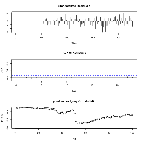 

In the first line, the % Rpush instruction loads objects for use in R. The % R instruction in the second line calls the code in the R language format. This construct works in IPython Notebook .
From the graphs above, you can see that the residuals are independent (this can be seen from the ACF ). In addition, from the graph of Q-statistics, it can be noted that at all points the value of p-value is greater than the significance level, it can be concluded from this that the residuals are, most likely, “white noise”.

Forecasting

To run, you need to load the forecast library.

 forecast = importr('forecast') 

Output prediction results in two ways.

Method 1. This is to use the integration capabilities of IPython and R. Which was shown in the previous section:

 %R plot(forecast(model))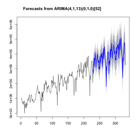 

Method 2. The second way is to make a forecast using the forecast library, and then translate the result into a time series of pandas and display them on the screen. The code that will execute is written below:

 f = forecast.forecast(model) #  pred = [i[1] for i in f[3].iteritems()] #  dt = date_range(w.index[-1], periods=len(pred)+1,freq='W')[1:] #    pr = Series(pred, index = dt) #   TimeSeries 

Now we will display the result on the screen.

 w.plot(figsize=(12,6)) pr.plot(color = 'red') 

Conclusion

As a conclusion, I would like to note that for a more accurate analysis of seasonality, you need to have data from 7-10 seasons. In addition, I would like to say a big thank you to werwooolf for the assistance in the process of preparing the article.
In this article, I tried to show how to build a seasonal ARIMA model, and also showed how you can use a bunch of R and Python languages for data analysis. I think experts will find out how to apply the described bundle effectively, in a single and different language.