Poisson process simulation

Introduction

One of the most important processes observed in nature is the Poisson point process. Therefore, it is important to understand how such processes can be modeled. Modeling methods vary depending on the type of Poisson point process, i.e. the space in which the process proceeds and the homogeneity or heterogeneity of the process. We will not be interested in the development of a Poisson point flow or with important applications of it in various fields. To make this material interesting, the reader is strongly advised to read the relevant sections in Feller (1965) and Sinlar (1975) for the main theory and some sections in Trivedi (1982) for IT applications.

In the first step, we define the Poisson process on [0; + ∞). The process is completely determined by a family of random events that occur at certain random times 0 <T1 <T2 <... These events can relate to a variety of things, such as bank robbery, the birth of five twins, and an accident involving a Montreal taxi. If N (t1, t2) is the number of events that occurred during the time interval (t1, t2), then the following two conditions are often met:

• For disjoint intervals (t1, t2) and (t3, t4), the random variables N (t1, t2) and N (t3, t4) are independent
• N (t1, t2) is distributed as well as N (0, t2-t1), i.e. the distribution of the number of events for a certain time depends only on the length of this interval.

The surprising fact is that these two conditions imply that all random variables N (t1, t2) are distributed according to the Poisson law and that there is a nonnegative constant λ such that N (t, t + a) is distributed according to the law Po (λa ) for any non-negative t and a> 0. See, for example, Feller (1965). Thus, the Poisson distribution occurs quite naturally.
')
The previous concept can be generalized to R ^d . Let A be some subset of R ^d , and N a random variable taking only integer values. Let X ₁ , ... X _N be a set of random vectors taking a value in A. Then we say that X _i define a uniform or homogeneous Poisson process on A if

• For any finite set of pairwise disjoint subsets of the set A _{i of} finite volume of the event N (A ₁ ), ..., N (A _{k are} independent
• For any Borel subset B of set A, the distribution N (B) depends only on the volume of set B

Translator's note: It would be better to use the word "measure", but for those who are not keen on mathematics, then they would have to explain with a dozen pages, or even more.

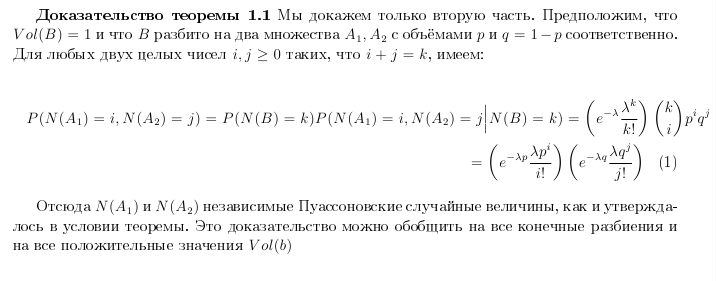
Again, these assumptions imply that all N (B) are distributed according to the law P (λVol (B)) for some non-negative λ, which we call intensity, or intensity parameter of a homogeneous Poisson process on A. Examples of such processes in a multidimensional Euclidean space include bacteria on a petri dish and murder sites in Houston.

Simulation of homogeneous Poisson processes

If we need to model a uniform Poisson process on a set A belonging to R _d , then we need to generate a certain number of random vectors X _i from A. By Theorem 1.1, this can be done as follows:

N λVol(A)
X1,..,XN,
RETURN 1,...,N

To generate the value of N, it is useless to use an algorithm with an average complexity of O (1), since at the end of the algorithm, we will spend at least Ω (n) operations. Therefore, if this algorithm is used, it is strongly recommended to generate a Poisson random variable with a very simple algorithm (with an average time growing as O (λ)). For certain sets A, you can use other methods that do not require explicit generation of a Poisson random variable. There are three cases that we use to illustrate this.

1. A = [0; + ∞)
2. A - circle
3. A - rectangle

To do this, we need an interesting connection between the Poisson process and the exponential distribution.


Theorem 1.2 suggests the following method for simulating a uniform Poisson process on A = [0; + ∞)

T = 0 ( "")
k = 0 ( )
REPEAT

k = k + 1
T = T + E/λ
T[k] = T
UNTIL ( ; )

This algorithm is easy to implement, since there is no need to generate Poisson random variables. For other simple sets A, there are trivial generalizations of Theorem 1.2. For example, when A = [0, t] x [0,1], where t can be equal to infinity, 0 <T1 <T2 <... is a uniform Poisson process with intensity λ and U1, U2, ... is a sequence of independent equally distributed uniformly on [0,1] of random variables, then (T1, U1), (T2, U2), ... determine the Poisson process with intensity λ on A.

Example 1.1.

Uniform Poisson process on the unit circle
If A is a circle with a unit radius, then different properties of the uniform Poisson process can be used to obtain several methods of generation (which are generalized to d-dimensional spheres). Let λ be the desired intensity.
First, we could simply generate a random Poisson value N with the parameter λπ, and then return a sequence of N independent identically distributed uniformly on the unit circles of vectors. If we apply the order statistics method proposed by Theorem 1.2, then a Poisson random variable is obtained implicitly. For example, going to the polar coordinates (R, φ), we note that for a uniform Poisson process, R and φ are independent, and the random variable R has a density of 2r, r varies from 0 to 1, and φ is uniformly distributed on [0; 2π]. Thus, we can proceed as follows: Generate a uniform Poisson process 0 <φ1 <φ2 <... <φN with the intensity parameter λ / (2π) to [0; 2π] by the exponential method and return (φ1, R1), ..., (φN, RN), where Ri are independent identically distributed random variables with a density of 2r on [0; 1], which can be generated by taking a maximum of two random variables uniformly distributed on [0; 1]. There is no special reason to apply the exponential method to the corners. In the same way we could pick up the radii. Unfortunately, ordinal radii do not form a one-dimensional uniform Poisson process on [0; 1]. However, they nonetheless form a non-uniform Poisson process, and the generation of such processes will be discussed in the next section.

Heterogeneous Poisson processes

There are situations when events occur at "random times", but some moments are more possible than others. This is a case of arrivals at intensive care centers, job offers at computer centers and injuries to NHL players. For these cases, a very good model is the model of the inhomogeneous Poisson process, defined here for the sake of convenience at [0; + ∞). This is the most important case, since time is most often a “running variable”.
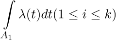
The inhomogeneous Poisson process on [0; + ∞) is determined by a nonnegatively defined intensity function Λ (t), which can be considered as some kind of density with the difference that its integral over [0; + ∞) is not necessarily equal to 1 (usually, it diverges ). The process is defined by the following property: for any finite collection of non-intersecting intervals A1, A2, ..., Ak, the number of events occurring in these intervals (N1, ..., Nk) are independent Poisson random variables with parameters

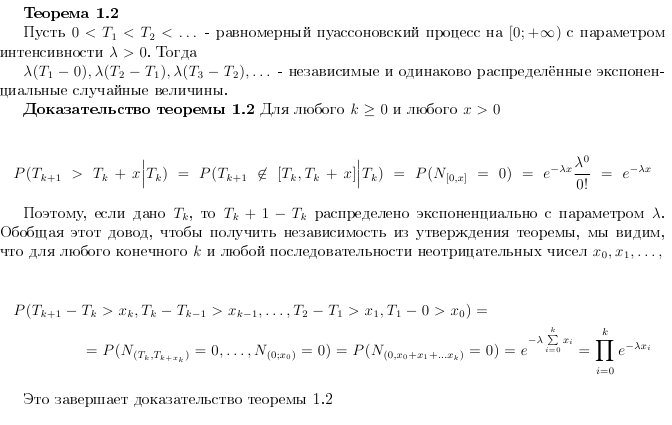
Now consider how such processes can be modeled. In the simulation, we understand that the points in time when events occur, 0 <T1 <T2 <... must be specified in ascending order. Much work on modeling inhomogeneous Poisson processes was done by Lewis and Schedler (1979). This entire section is a revised version of their work. It is interesting to observe that the general principles of generation of continuous random variables can be extended: we will see that there are analogues by the method of inversion, deviation, and composition.
The role of the distribution function will be taken by the integrated intensity function.

We begin by noting that if T _n = T, then T _{n + 1} -T _n has a distribution function

if the function Λ (t) increases unboundedly with increasing t. This follows from the fact that



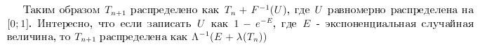
In other words, we need to convert Λ. Formally, we have (see also Sinlar (1975) or Brettley, Fox and Schrage (1983)) an algorithm based on inverting the integral of the intensity function (inversion method)

T = 0 ( )
k = 0 ()
REPEAT
E
k = k+1
T = T + InvΛ(E+Λ(T)), (InvΛ - Λ)
T[k] = T
UNTIL False

Example 1.2. Homogeneous Poisson process

For the special case of λ (t) = λ, Λ (t) = λt, it is easy to see that InvΛ (E + Λ (T)) = T + E / λ, as a result of which we again obtain the exponential method.

Example 1.3.

To simulate the morning flow of cars before the rush hour, we can sometimes take λ (t) = t, then Λ (t) = t ^ 2/2 and get a step

If the intensity function can be represented as the sum of the intensity functions, i.e. ,

0 <T _i1 <T _i2 <... T _in are independent implementations of individual inhomogeneous Poisson processes, then the combined ordered sequence forms the implementation of a non-uniform Poisson process with intensity function λ (t). This refers to the composition method, but the difference now is that we need implementations of all the components of the process. Decomposition can be used when there is a natural decomposition dictated by the analytical form λ (t). Since the main operation in merging processes is to take the minimum value of n processes, for large n, storage of points of time on an heap of n elements can give an advantage.

As a result, we obtain the composition method:

T[1,1],...,T[n,1] n
T = 0 ( )
k = 0
REPEAT
T[i,j]
k = k + 1
T[k] = T[i,j]
T[i,j+1]
UNTIL False

The third general principle is the principle of thinning (Lewis and Schedler, 1979). Similarly to what happens in the deviation method, we assume that there is a light dominant intensity function λ (t) <= μ (t) for any t.

Then the idea is to generate a homogeneous Poisson process on a part of the positive half-plane between 0 and μ (t), then consider a homogeneous Poisson process under λ and, finally, return the x-components of events in this process. This requires the following theorem.




Now consider the thinning method of Lewis and Schedler:

T = 0
k = 0
REPEAT
Z, μ, T. T = Z
[0;1] U
IF U <= λ(Z)/μ(Z)
THEN k = k + 1, X[k] = T
UNTIL False

It is argued that the sequence X _k so generated forms an inhomogeneous Poisson process with an intensity function λ. Note that we took the inhomogeneous process 0 <Y1 <Y2 <... with the intensity function μ and removed some points. As far as we know, (Y _i , U _i μ (Y _i ) is a homogeneous Poisson process with unit intensity on the curve, if U _{i is} independent randomly distributed uniformly on [0; 1] random variables by virtue of Theorem 1.3. Thus, the subsequence on the curve λ defines a homogeneous Poisson process with unit intensity on this curve (part 3. of Theorem 1.3). Finally, taking the x-coordinates of only this subsequence gives us a non-uniform Poisson process with an intensity function λ.
Inhomogeneous Poisson process with an intensity function μ is usually modeled by the inversion method.

Example 1.4. Cyclic intensity function

The following example also belongs to Lewis and Schedler (1979). Consider a function with cyclic intensity λ (t) = λ (1 + cos (t)) with an obvious choice of the dominant function μ = 2λ.

Then the simulation algorithm will take the form:

T = 0
k = 0
REPEAT
E c 1
T = T + E/(2λ)
[0;1] U
IF U <= (1+cos(T))/2
THEN k = k + 1, X[k] = T
UNTIL False

Needless to say, we can use the two policemen theorem here to avoid calculating the cosine in most cases.

The final word on the efficiency of the algorithm when a non-homogeneous Poisson process on the set [0, t] is modeled. The average number of events that is necessary from the dominant process is equal to while the average number of returned random variables is
The ratio of average values ​​can be considered as an objective measure of efficiency, comparable in the spirit of the deviation constant in the standard deviation method. Note that we cannot use the average value of the ratio, since, in general, it would be equal to infinity due to the positive probability that no value will return.